Socio-Political

The most recent and complete socio-political model documentation is available on Pardee's website. Although the text in this interactive system is, for some IFs models, often significantly out of date, you may still find the basic description useful to you.

A substantial portion of the socio-political model of IFs is scattered throughout the other models. There are "policy handles" or intervention points throughout those models. For instance, in the population model, multipliers on the total fertility rate can reflect policy decisions (although they can also reflect the model user's judgment concerning social changes in the country or region, independent of policy). Patterns of regulation, subsidy, tax incidence, and provision of state services are so diffuse and complicated that we resort to looking at their aggregate consequences through various "policy handles" rather than trying to represent them explicitly.

For more information on this module, please use the links below or read more at Socio-Political Equations Overview.

Structure and Agent System: Socio-Political

System/Subsystem	Socio-political
Organizing Structure	Social fabric
Stocks	Levels of human well-being and institutional development (human and social capital)   Cultural structures
Flows	Social expenditures   Value change
Key Aggregate  Relationships  (illustrative, not comprehensive)	Growth in literacy and human development;   Democratic development, state failure
Key Agent-Class Behavior  Relationships (illustrative, not comprehensive)	Government efforts to develop human capital through spending on health, education, R&D

Unlike the use of cohort-component structures in demographics and of markets and social accounting matrices for economics, there is no standard organizing structure that is widely used for representing socio-political systems. In the context of the TERRA project, IFs developed a multi-component approach to structure that might be called the "social fabric" (a la Robert Pestel).

Although representation of agent-class behavior would be of special interest in a socio-political module, most relationships in IFs remain at the level of aggregate specifications.

Dominant Relations: Socio-political

Domestic Socio-Political Change: Dominant Relations

Social and political change occurs on three dimensions (social characteristics or individual life conditions, values, socio-political institutions and process). Although GDP per capita is strongly correlated with all dimensions of change, it might be more appropriate to conceptualize a syndrome or complex of developmental change than to portray an economically-driven process.

For causal diagram see Socio-Political Flow Charts Overview.

For equations see, for example, Socio-Political Equations Overview.

Key dynamics are directly linked to the dominant relations:

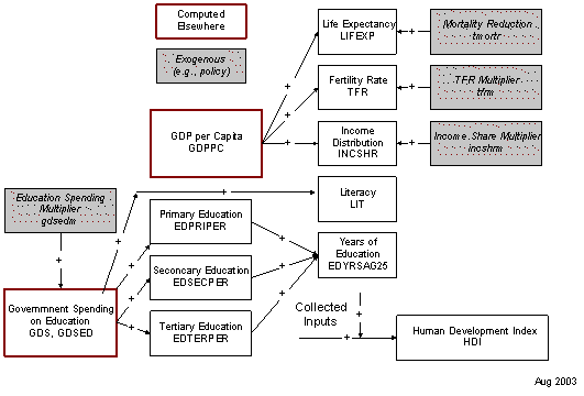
• The model computes some key social characteristics/life conditions, including life expectancy and fertility rates in the demographic model, but the user can affect them via multipliers (mortm, tfrm). Literacy rate is an endogenous function of education spending, which the user can influence (via gdsm).
• The model computes value or cultural change on three dimensions: traditional versus secular-rational, survival versus self-expression, and modernism versus postmodernism, which the user can affect via additive factors (tradsrateadd, survseadd, matpostradd).
• Freedom, democracy (the POLITY measure), autocracy, economic freedom, and the status of women are all computed endogenously but can all be shifted by the user via multipliers (freedomm, democm, autocm, econfreem, gemm)

Domestic Socio-Political Change: Selected Added Value

The larger socio-political model provides representation and control over government spending on education, health, the military, R&D, foreign aid, and a residual category. Military spending is linked to interstate politics, both as a driver of threat and as a result of action-and-reaction based arms spending. The sub-model provides aggregated indicators of the physical quality of life and the human development index.

Socio-political Flow Charts

SP1.gif

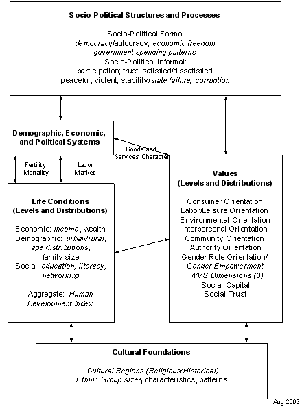
The social and political module represents a complex of interacting structures and processes. These include:

• The various social characteristics or life conditions of individuals
• Human values, beliefs, and orientations’
• Social and political structures, informal as well as formal
• Social and political processes, both domestic and international

Cultural foundations frame all of these components. And all of the components interact closely with human demographic and economic systems.

The socio-political elements of IFs are among the most dynamically evolving aspects of the overall modeling system. Much, but not everything in the above figure has been fully represented yet within IFs; the figure indicates direction of development and shows implemented elements in italics.

For more, please read the links below.

Social Characteristics: Life Conditions

Individuals are the foundations of society. Many social indicators are actually aggregated indicators of their condition. The Human Development Index (HDI) is a widely-used summary measure of that life condition, based on life expectancy, educational attainment, and GDP per capita.

Sp2.gif

Physical Quality of Life (PQLI)

The Overseas Development Council (then under the leadership of Jim Grant) developed and publicized a measure of (physical) quality of life (the PQLI) many years ago. It combines literarcy rate, infant mortality rate, and life expectancy, using scales from the lowest to the highest values in the global system. It weights the three scales equally. The literacy rate is, in turn, a function of the per capita spending levels on education, estimated cross-sectionally. In many respects the PQLI was a predecessor of the human development index (HDI).

Physical Quality of Life

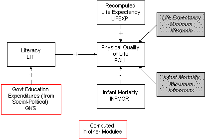
Based on country/region-specific Physical Quality of Life, it is possible to compute world quality of life (WPQLI) and the North-South gap in quality of life (NSPQLI). Given country-specific literacy rates, it is also possible to compute world literacy (WLIT).

Income Distribution

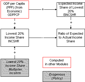
Income distribution is represented by the share of national income earned by the poorest 20 percent of the population. That share is obtained from data whenever possible, but is estimated from a cross-sectional relationship when necessary and changed over time by that relationship (the values tend, however, to be very stable both in the real world and in the model). Because initial conditions of variables affected by income share, such as fertility and mortality rates, already reflect existing income distributions, it is only the changes in that distribution relative to the expected value that the model uses in such relationships. A parameter (incshrm) is available to change income share and thus affect those variables influenced by it.

Sp4.gif

Social Characteristics: Networking

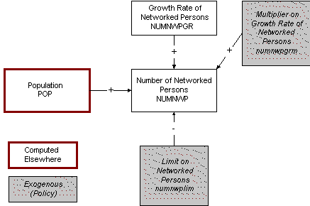
Being electronically networked is an increasingly important aspect of human life condition. The number of networked persons (NUMNWP) is a function primarily of the growth rate in that number (NUMNWPGR). It is ultimately constrained, however, by the size of the population and by the number of connections and organizational memberships that people can have (numnwplim). The growth in networked person number slows as it approaches the ultimate limit. The model user can affect the growth pattern via a multiplier on the growth rate (numnwpgrm).

This approach was added to IFs during the TERRA project and draws on the thinking of Tom Tesch and Pol Descamps.

Sp5.gif

Social Values and Cultural Evolution

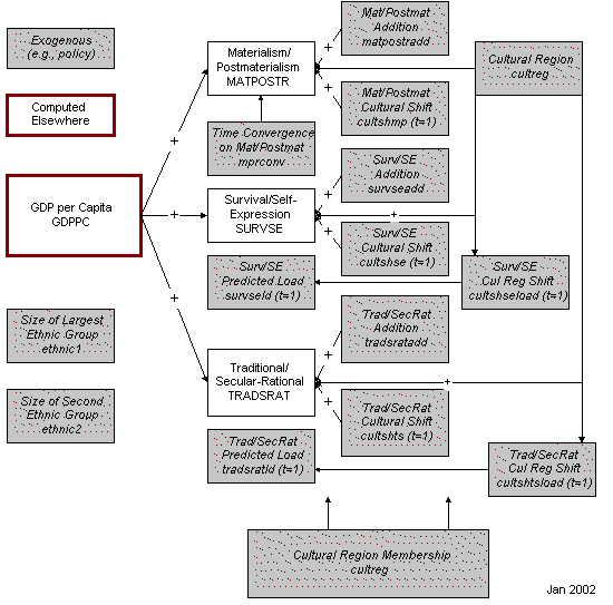
IFs computes change in three cultural dimensions identified by the World Values Survey (Inglehart 1997). Those are dimensions of materialism/post-materialism, survival/self-expression, and traditional/secular-rational values.

Inglehart has identified large cultural regions that have substantially different patterns on these value dimensions and IFs represents those regions, using them to compute shifts in value patterns specific to them.

Levels on the three cultural dimensions are predicted not only for the country/regional populations as a whole, but in each of 6 age cohorts. Not shown in the flow chart is the option, controlled by the parameter "wvsagesw," of computing country/region change over time in the three dimensions by functions for each cohort (value of wvsagesw = 1) or by computing change only in the first cohort and then advancting that through time (value of wvsagesw = 2).

The model uses country-specific data from the World Values Survey project to compute a variety of parameters in the first year by cultural region (English-speaking, Orthodox, Islamic, etc.). The key parameters for the model user are the three country/region-specific additive factors on each value/cultural dimension (matpostradd, etc.).

Finally, the model contains data on the size (percentage of population) of the two largest ethnic/cultural groupings. At this point these parameters have no forward linkages to other variables in the model.

Sp6.gif

Social Organization and Change

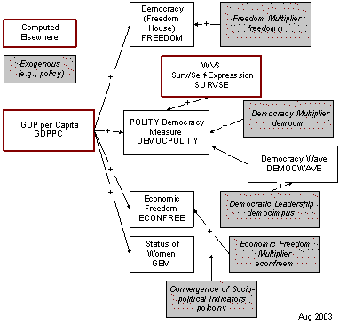
The sociopolitical module computes change in freedom (political and economic) and the status of women. For freedom it uses both the measure of the Freedom House and the combined measure for democracy (building on democracy and autocracy) of the POLITY project. It also computes a measure of economic freedom and of gender equality.

Sp7.gif

Social Organization: Stability/State Failure

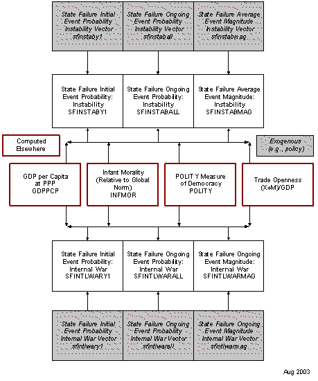
The State Failure project has analyzed the propensity for different types of state failures within countries, including those associated with revolution, ethnic conflict, genocide-politicide, and abrupt regime change (using categories and data pioneered by Ted Robert Gurr. Upon the advice of Gurr, IFs groups the first three as internal war and the last as political instability.

IFs uses the same primary variables (infant mortality, democracy, and trade openness) as the State Failure project to drive forecasts of the probability of individual events of state failure, of ongoing episodes of it, and of the magnitude of episodes. In addition, it allows the use in the formulation of GDP per capita and years of education. Many other linkages have been and can be explored, including cultural regions.

Sp8.gif

Government Spending

The economic submodel provides total government spending. Government spending by category begins as a simple product of total government consumption and fractional shares by spending category.

Spending by type (military, health, education, research and development, other, and foreign aid) is largely specified exogenously, building on the initial conditions for each country/region. In addition, an action-reaction (arms-race) dynamic can be established in military spending if the action-reaction switch is turned on. After adjustments to foreign aid and military spending, spending in all categories is re-normalized to equal total governmental spending.

Educational spending is further broken out of total educational spending. The user can shift the spending across three educational levels (primary, secondary, and tertiary) through the use of an educational multiplier.

Gs1.gif

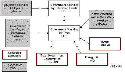
See also the specifications of detailed final demand and of international finance.

Socio-political Equations

Overview

A substantial portion of the policy model of IFs is scattered throughout the other models. There are "policy handles" or intervention points throughout those models. For instance, in the population model, multipliers on the total fertility rate can reflect policy decisions (although they can also reflect the model user's judgment concerning social changes in the country or region, independent of policy). Similarly, in the energy model, the multiplier on energy demand can represent conservation policy. Similarly, the ultimate energy resource base and the rate of resource discovery remain uncertain in part because they are subject to a wide range of government interventions - multipliers can introduce assumptions about such interventions. In the economic module, the level of trade protection is very clearly a policy parameter as is the multiplier on the tax rate. Patterns of regulation, subsidy, tax incidence, and provision of state services are so diffuse and complicated that we resort to looking at their aggregate consequences through various "policy handles" rather than trying to represent them explicitly.

IFs contains other categories of sociol-political activity, however, that it represents in more integrated fashion in the sociopolitical module as a four-dimensional social fabric: social characteristics/life condition, values, social structures (formal and informal), and social processes.

For help understanding the equations see Notation.

Socio-political Equations: Life Conditions

Literacy changes from the initial level for the region because of a multiplier (LITM).

$LIT_{\gamma }=\mathbf {LIT} _{\gamma }^{t=1}*LITM_{\gamma }$

The function upon which the literacy multiplier is based represents the cross#sectional rela"tionship globally between educational expenditures per capita (EDEX) from the government submodel and literacy rate (LIT). Rather than imposing the typical literacy rate on a region (and thereby being inconsistent with initial empirical values), the literacy multiplier is the ratio of typical literacy at current expenditure levels to the normal literacy level at initial expenditure levels. This formulation predates the development of an educational module that calculates the numbers of those with a primary education (one common definition of literacy). As that module is refined, we will likely derive literacy dynamics from it.

$LITM={\frac {AnalFunc(EDEX)}{AnalFunc(\mathbf {EDEX} ^{t=1})}}$

Educational expenditures (and thus implicitly literacy and labor efficiency) are tied back to the economic model via the economic production function.

Given life expectancy, literacy, and infant mortality levels from the mortality distribution, it is possible to compute the Physical Quality of Life Index (PQLI) that the Overseas Development Council developed (ODC, 1977: 147#154). This measure averages the three quality of life indicators, first normalizing each indicator so that it ranges from zero to 100. The normaliza"tion is not needed for literacy; for life expectancy it converts the range of approximately 28 (LIFEXPMIN) to 80 (LIFEXPMAX) years into 0 to 100; for infant mortality it converts the range of approximately 229 per thousand (INFMORMAX) to 9 per thousand (INFMORMIN) into 0 to 100.

$PQLI_{\gamma }={\frac {LIT_{\gamma }+{\frac {LIFEXP_{\gamma }-\mathbf {lifexpmin} }{LifExpMax-\mathbf {lifexpmin} }}*100+{\frac {\mathbf {infmormax} -MORDST_{\gamma ,c-1}}{\mathbf {infmormax} -InfMorMin}}*100}{300}}$

where

$LifExpMax=Max(LIFEXP_{\gamma }^{t})$

$InfMorMin=Min(INFMOR_{\gamma }^{t})$

For most users, the United Nations Development Program’s human development index (HDI) has replaced the PQLI as an integrated measure of life condition. It is a simple average of three sub-indices for life expectancy, education, and GDP per capita (using purchasing power parity). The life expectancy sub-index is the same as was used for the PQLI. The literacy sub-index is again the literacy rate. The GDP per capita index is a logged form that runs from a minimum of 100 to a maximum of $40,000 per capita. The measure in IFs differs slightly from the HDI version, because it does not put educational enrollment rates into a broader educational index with literacy; that will be changed as the educational model of IFs is better tested.

$HDI_{\gamma }={\frac {LifeExpInd_{\gamma }+LitInd+GDPInd}{3}}$

where

$LifeExpInd={\frac {LIFEXP_{\gamma }-LIFEXPMIN}{LIFEXPMAX-LIFEXPMIN}}$

$LitInd=LIT_{\gamma }/100$

$GDPInd={\frac {Log(GDPPCP_{\gamma }*1000)-Log(100)}{Log(40000)-Log(100)}}$

Although the HDI is a wonderful measure for looking at past and current life conditions, it has some limitations when looking at the longer-term future. Specifically, the fixed upper limits for life expectancy and GDP per capita are likely to be exceeded by many countries before the end of the 21st century. IFs has therefore introduced a floating version of the HDI, in which the maximums for those two index components are calculated from the maximum performance of any state in the system in each forecast year.

$HDIFLOAT_{\gamma }={\frac {LifeExpInd_{\gamma }+LitInd+GDPInd}{3}}$

where

$LifeExpInd={\frac {LIFEXP_{\gamma }-LIFEXPMIN}{HDILIFEMAXFLOAT-LIFEXPMIN}}$

$LitInd=LIT_{\gamma }/100$

$GDPInd={\frac {Log(GDPPCP_{\gamma }*1000)-Log(100)}{Log(GDPPCPMAX)-Log(100)}}$

The floating measure, in turn, has some limitations because it introduces relative attainment into the equation rather than absolute attainment. IFs therefore uses still a third version of the HDI, one that allows the users to specify probable upper limits for life expectancy and GDPPC in the twenty-first century. Those enter into a fixed calculation of which the normal HDI could be considered a special case.

$HDI21stFIX_{\gamma }={\frac {LifeExpInd_{\gamma }+LitInd+GDPInd}{3}}$

where

$HDILIFEMAX21=\mathbf {hdilifemaxf}$

$LifeExpInd={\frac {LIFEXP_{\gamma }-LIFEXPMIN}{HDILIFEMAX21-LIFEXPMIN}}$

$LitInd=LIT_{\gamma }/100$

$Log(GDPPCP21)=Log(\mathbf {hdigdppcmax} *1000)$

$GDPInd={\frac {Log(GDPPCP_{\gamma }*1000)-Log(100)}{Log(GDPPCP21)-Log(100)}}$

It is useful to compute several additional global indicators, a world physical quality of life index (WPQLI), a world life expectancy (WLIFE), a world literacy rate (WLIT), and a North#South gap index or ratio of quality of life in the "developed -D" regions to the "less developed-L" regions (NSPQLI).

$WPQLI={\frac {\sum ^{R}PQLI_{\gamma }*POP_{\gamma }}{WPOP}}$

$WLIFE={\frac {\sum ^{R}LIFEXP_{\gamma }*POP_{\gamma }}{WPOP}}$

$WLIT={\frac {\sum ^{R}LIT_{\gamma }*POP_{\gamma }}{WPOP}}$

$NSPQLI={\frac {\frac {\sum ^{D}PQLI_{\gamma }*POP_{\gamma }}{\sum ^{D}POP_{\gamma }}}{\frac {\sum ^{L}PQLI_{\gamma }*POP_{\gamma }}{\sum ^{L}POP_{\gamma }}}}$

Socio-political Equations: Income Distribution

The income share of the poorest 20 percent of the population (INCSHR) depends on the GDP per capita at PPP (GDPPCP) and on an exogenous income share multiplier (incshrm).

$INCSHR_{\gamma }^{t}=INCSHR_{\gamma }^{t}*{\frac {AnalFunc(GDPPCP_{\gamma })}{AnalFunc(GDPPCP_{\gamma }^{t-1})}}*\mathbf {incshrm_{\gamma }}$

The introduction of different household types into the social accounting matrix structure of IFs made possible the computation of a more sophisticated measure of income distribution tied directly to the model’s computation of household income (HHINC) and household size (HHPOP) by type. A domestic Gini value (GINIDOM) is calculated from a function that uses the normal Lorenz curve foundation for Gini indices. Because that function can calculate values that are quite different from the empirical initial values, a ratio of the empirical value to the initial computed value (GINIDOMRI) is used for scaling purposes. The model’s formulation of the relative household income levels of different household types, and therefore the calculation of a domestic GINI based on those income levels, are in early versions and are still rather crude.

$GINIDOM_{\gamma }^{t}=GINIFUN(HHINC_{R,S},HHPOP_{R,S})*GINIDomRI_{\gamma }^{t-1}$

where

$GINIDomRI_{\gamma }^{t-1}={\frac {GINIDOM_{\gamma }^{t-1}}{GINIFUN(HHINC_{R,S}^{{\gamma }-1},HHPOP_{R,S}^{t-1})}}$

One value of a domestic Gini calculation is that it, in turn, makes possible the calculation of the percentage of population living on less than one dollar per day (INCOMELT1) or two dollars per day (INCOMELT2). Functions were estimated linking GDP per capita at purchasing power (GDPPCP) and the Gini index to those percentages. Again, IFs uses initial conditions for scaling purposes.

$INCOMELT1_{\gamma }^{t}=AnalFunc(GDPPCP_{\gamma },GINIDOM_{\gamma })*INCOMELT1RI_{\gamma }^{t-1}$

where

$INCOMELT1RI_{\gamma }^{t-1}={\frac {\mathbf {INCOMELT1} ^{t-1}{\gamma }}{AnalFunc(GDPPCP_{\gamma }^{\gamma -1},GINIDOM_{\gamma }^{t-1})}}$

$INCOMELT2_{\gamma }^{t}=AnalFunc(GDPPCP_{\gamma },GINIDOM_{\gamma })*INCOMELT2RI_{\gamma }^{t-1}$

where

$INCOMELT2RI_{\gamma }^{t-1}={\frac {INCOMELT2_{\gamma }^{t-1}}{AnalFunc(GDPPCP_{\gamma }^{\gamma -1},GINIDOM_{\gamma }^{t-1})}}$

IFs also calculates a global Gini index across all countries/regions in the model, again using the standard Lorenz curve approach to areas of inequality and equality. It does not yet take into account intra-regional income differentials, but the foundation is now in place to do so.

$GINI_{\gamma }^{t}=GINIFUN(GDP_{R},POP_{R})$

The user interface of IFs now uses the same Lorenz-curve approach to allow the user to calculate a specialized-display GINI for any variable that can be represented across all countries/regions of the model.

Social Equations Networking

The focal point of this portion of the model is on the computation of the total number of networked persons (NUMNWP). The rate of growth in that number (NUMNWPGR) is subject to several forces. The initial value of that rate is set in the data preprocessor of the model from empirical data. When no data are available for a country or region, the rate is set at a level determined via a cross-sectional relationship between GDP per capita (PPP) and portion of population networked.

$NUMNWP_{\gamma }=NUMNWP_{\gamma }^{t-1}*(1+NumNwGR_{\gamma }^{t})$

where

$NumNwGR_{\gamma }^{t}=NUMNWPGR_{\gamma }^{t-1}*({\frac {nwplm-NUMNWP_{\gamma }^{t-1}}{nwplm-NUMNWP_{\gamma }^{t-1}}})^{2}*numnwpgrm$

$nwplm=numnwplim*POP_{\gamma }$

Over time the growth rate of networked persons is subject to a saturating function, as the actual number of networked persons approaches a limit. The limit is set by an exogenous multiplier (numnwplim) on total population; networked persons can exceed total population because of multiple affiliations of individuals (households, NGOs, companies). The user of the model can accelerate or de-accelerate the process of networking via a multiplier on the growth rate (numnwpgrm).

Although of interest in its own right, the number of networked persons is also carried forward in the model to the production function of the economy.

Socio-political Equations: Values

IFs computes change in three cultural dimensions identified by the World Values Survey (Inglehart 1997). Those are dimensions of materialism/post-materialism (MATPOSTR), survival/self-expression (SURVSE), and traditional/secular-rational values (TRADSRAT). On each dimension the process for calculation is somewhat more complicated than for freedom or gender empowerment, however, because the dynamics for change in the cultural dimensions involves the aging of population cohorts. IFs uses the six population cohorts of the World Values Survey (1= 18-24; 2=25-34; 3=35-44; 4=45-54; 5=55-64; 6=65+). It calculates change in the value orientation of the youngest cohort (c=1) from change in GDP per capita at PPP (GDPPCP), but then maintains that value orientation for the cohort and all others as they age. Analysis of different functional forms led to use of an exponential form with GDP per capita for materialism/postmaterialism and to use of logarithmic forms for the two other cultural dimensions (both of which can take on negative values).

$MATPOSTR_{\gamma ,c-1}=\mathbf {MATPOSTR} _{\gamma ,c-1}^{t-1}*{\frac {AnalFunc(GDPPCP_{\gamma })}{AnalFunc(GDPPCP_{\gamma }^{t-1})}}+\mathbf {CultShMP} _{\gamma -cultural}^{t}+\mathbf {matpostradd} _{\gamma }^{t}$

where

$\mathbf {CultShMP} _{\gamma -cultural}^{t}=F(\mathbf {MATPOSTR} _{\gamma ,c-1}^{t-1},AnalFunc(GDPPCP_{\gamma }^{t-1})$

$SURVSE_{\gamma ,c-1}=\mathbf {SURVSE} _{\gamma ,c-1}^{t-1}*{\frac {AnalFunc(GDPPCP_{\gamma })}{AnalFunc(GDPPCP_{\gamma }^{t-1})}}+\mathbf {CultShSE} _{\gamma -cultural}^{t}+\mathbf {survseadd} _{\gamma }^{t}$

where

$CultShSE_{\gamma -cultural}^{t}=F(\mathbf {SURVSE} _{\gamma ,c-1}^{t-1},AnalFunc(GDPPCP_{\gamma }^{t-1})$

$TRADSRAT_{\gamma ,c-1}=\mathbf {TRADSRAT} _{\gamma ,c-1}^{t-1}*{\frac {AnalFunc(GDPPCP_{\gamma })}{AnalFunc(GDPPCP_{\gamma }^{t-1})}}+\mathbf {CultShTS} _{\gamma -cultural}^{t}+\mathbf {tradsratadd} _{\gamma }^{t}$

where

$\mathbf {CultShTS} _{\gamma -cultural}^{t}=F(\mathbf {TRADSRAT} _{\gamma ,c-1}^{t-1},AnalFunc(GDPPCP_{\gamma }^{t-1})$

The user can influence values on each of the cultural dimensions via two parameters. The first is a cultural shift factor (e.g. CultSHMP) that affects all of the IFs countries/regions in a given cultural region as defined by the World Value Survey. Those factors have initial values assigned to them from empirical analysis of how the regions differ on the cultural dimensions (determined by the pre-processor of raw country data in IFs), but the user can change those further, as desired. The second parameter is an additive factor specific to individual IFs countries/regions (e.g. matpostradd). The default values for the additive factors are zero.

Some users of IFs may not wish to assume that aging cohorts carry their value orientations forward in time, but rather want to compute the cultural orientation of cohorts directly from cross-sectional relationships. Those relationships have been calculated for each cohort to make such an approach possible. The parameter (wvsagesw) controls the dynamics associated with the value orientation of cohorts in the model. The standard value for it is 2, which results in the "aging" of value orientations. Any other value for wvsagesw (the WVS aging switch) will result in use of the cohort-specific functions with GDP per capita.

Regardless of which approach to value-change dynamics is used, IFs calculates the value orientation for a total region/country as a population cohort-weighted average.

IFs uses an approach that is similar to the one for literacy in order to estimate the future of another measure created by the United Nations Development Program, one called the Gender Equity Measure (GEM). The closer the values of that measure approach "1", the closer women are to men in political and social power.

$GEM_{\gamma }=GEM_{\gamma }^{t-1}*{\frac {AnalFunc(GDPPC_{\gamma })}{AnalFunc(GDPPC_{\gamma }^{t-1})}}$

Socio-political Equations: Structures or Institutions

IFs endogenizes level of freedom (FREEDOM), based on the Freedom House measures, by linking change from initial conditions to GDP per capita at purchasing power parity in an analytic function. For discussion of the relationship between GDP and democracy, see Londregran and Poole (1996) and Przeworski and Limongi (1997). The latter view it as a probabilistic relationship in which there are a variety of reasons (often external pressure) at all levels of economic development for the conversion of dictatorships to democracies and in which the conversion of democracies to dictatorships occurs commonly at low but not high levels of development. That pattern creates a positive correlation between economic development and democratic government. A multiplier in freedom level (freedomm) increases or decreases the level of freedom.

$FREEDOM_{\gamma }=FREEDOM_{\gamma }^{t-1}*{\frac {AnalFunc(GDPPCP_{\gamma })}{AnalFunc(\mathbf {GDPPCP} _{\gamma }^{t-1})}}*\mathbf {freedomm} _{\gamma }$

The Economic Freedom Institute (with leadership from the Fraser Institute; see Gwartney and Lawson with Samida, 2000) have also introduced a measure of economic freedom. IFs represents that in similar fashion.

$ECONFREE_{\gamma }=ECONFREE_{\gamma }^{t-1}*{\frac {AnalFunc(GDPPCP_{\gamma })}{AnalFunc(GDPPCP_{\gamma }^{t-1})}}*\mathbf {econfreem} _{\gamma }$

The POLITY project provides an alternative to the freedom house measure of freedom or democracy level. In fact, it provides multiple variables related to political system. IFs EARLIER included formations of two of those, democracy (DEMOC) and autocracy (AUTOC). They worked in completely analogous fashion.

$DEMOC_{\gamma }=DEMOC_{\gamma }^{t-1}*{\frac {AnalFunc(GDPPCP_{\gamma })}{AnalFunc(GDPPCP_{\gamma }^{t-1})}}*\mathbf {democm} _{\gamma }$

$AUTOC_{\gamma }=AUTOC_{\gamma }^{t-1}*{\frac {AnalFunc(GDPPCP_{\gamma })}{AnalFunc(GDPPCP_{\gamma }^{t-1})}}*\mathbf {autocm} _{\gamma }$

More recently, IFs has (1) combined the two Polity project measures into a single one as is often done with the Polity measures, setting POLITYDEMOC equal to democracy – autocracy + 10, a measure that runs from 0 to 20; (2) introduced a more complicated, multi-level forecast for the new measure.

Specifically, the project identified three levels of analysis for factors that affect democratic change: domestic, regional, and systemic. At each of the three levels there are multiple factors that can affect democracy within states. At the domestic level we can identify two categories of factors in particular:

• GDP per capita. This variable correlates highly with almost all measures of social condition; GDP provides the resources for democratization and other social change.
• values/culture. Values clearly do differ across countries and regions of the world and almost certainly affect propensity to democratize.

At the regional level (or, more accurately, the "swing-states" level) we can also identify three prospective drivers:

• world average effects. It is possible that the world average exerts a pull-effect on states around the world (for instance, increasingly globalization could lead to homogenization of a wide variety of social structures around the world).
• swing states effects. Some states within regions quite probably affect/lead others (obviously the former Soviet Union was a prime example of such a swing state within its sphere of influence, but there is reason to believe in lesser and less coercive effects elsewhere).
• regional average. States within a region possibly affect each other more generally, such that "swing states" are moved by regional patterns and not simply movers of them.

At the system level we identify three:

• systemic leadership impetus. It is often suggested that the United States and other developed countries can affect democratization in less developed countries, either positively or negatively
• snowballing of democracy (Huntington 1991). The wave character of democratization suggests that there may be an internal dynamic, a self-reinforcing positive feedback loop, of the process globally, partially independent of other forces that act on the process. Such a conclusion is consistent with the fact that idea spread and global regime development influence many types of social change (Hughes 2001)
• miscellaneous other forces. Historic analysis would identify world war, economic depression, and other factors to explain the global pattern of democratization, especially the surge or retreat of waves.

A project document prepared for the CIA’s Strategic Assessment Group (SAG) analyzed historic data and, in cooperation with David Epstein and Larry Diamond, fit an approach to it that cut across these three levels (see Hughes 2002: 59-74 for elaboration and documentation of the empirical work). The empirical work is not documented again here. The work did not find significant and consistent regional level effects, however, and the regional variables are therefore normally turned off.

The resulting formulation uses the domestic level as an initial base calculation because it is the empirically strongest piece, and later adds (optionally) the regional level effects and the systemic effects. The base calculation is further tied to the actual empirical levels in the initial year of the run, with the impact of the driving variables being felt only in change of those levels. An ‘expected" democracy level (DEMOCEXP) is computed using an analytic function that uses GDP per capita at purchasing power parity (GDPPCP) and the World Value Survey’s survival and self-expression dimension (SURVSE). These were found quite powerful in their level of correlation with democracy and the WVS dimension, interestingly, carries a cultural component into the formulation. The user can further modify this basic formulation with an exogenous multiplier (democm).

$DEMOCPOLITYBase_{\gamma }^{t}=\mathbf {DEMOCPOLITY} _{\gamma }^{t-1}*{\frac {DEMOCEXP_{\gamma }^{t}}{DEMOCEXP_{\gamma }^{t-1}}}*\mathbf {democm} _{\gamma }^{t}$

where

$DEMOCEXP_{\gamma }^{t}=AnalFunc(GDPPCP_{\gamma }^{t},SURVSE_{\gamma }^{t})$

It is also useful to have a separate calculation of the empirically strongest piece of the formulation, namely the domestic effects, but without any adjustment to the initial empirical values. The expected democracy variable (DEMOCEXP) carries that. It can be compared with the fully computed values to see the degree to which there may be tension in countries between democracy levels that GDP per capita and values would predict, on the one hand, and those that are in the initial data. The greatest tension levels tend to be in the Middle Eastern countries, where decmocracy is considerably below "expected" levels.

The initial conditions of democracy in countries carry a considerable amount of idiosyncratic, country-specific influence, much of which can be expected to erode over time. Therefore a revised base level is computed that converges over time from the base component with the empirical initial condition built in to the value expected purely on the base of the analytic formulation. The user can control the rate of convergence with a parameter that specifies the years over which convergence occurs (polconv) and, in fact, basically shut off convergence by sitting the years very high.

if $\mathbf {sweffects} =1$

then $SwingEffects_{\gamma }^{t}=timeadj*\mathbf {swingstsdem} _{\gamma -Swinger,p-1}*(WDemoc^{t-1}-DEMOCPOLITY_{\gamma -Swingee}^{t-1})+timeadj*\mathbf {swingstsdem} _{\gamma -Swinger,p-2}*(DEMOCPOLITY_{\gamma -Swinger}^{t-1}-DEMOCPOLITY_{\gamma -Swingee}^{t-1})+timeadj*\mathbf {swingstsdem} _{\gamma -Swinger,p-3}*(RgDemoc-DEMOCPOLITY_{\gamma -Swingee}^{t-1})$

where

$timeadj=.2$

$WDemoc^{t-1}={\frac {\sum ^{R}DEMOCPOLITY_{\gamma }^{t-1}}{R}}$

else

$SwingEffects_{\gamma }^{t}=0$

On top of the country-specific calculation sits the (optional) regional or swing state effect calculation (SwingEffects), turned on by setting the swing states parameter (swseffects) to 1. The swing effects term has three components. The first is a world effect, whereby the democracy level in any given state (the "swingee") is affected by the world average level, with a parameter of impact (swingstdem) and a time adjustment (timeadj) . The second is a regionally powerful state factor, the regional "swinger" effect, with similar parameters. The third is a swing effect based on the average level of democracy in the region (RgDemoc).

David Epstein of Columbia University did extensive estimation of the parameters (the adjustment parameter on each term is 0.2). Unfortunately, the levels of significance were inconsistent across swing states and regions. Moreover, the term with the largest impact is the global term, already represented somewhat redundantly in the democracy wave effects. Hence, these swing effects are normally turned off and are available for optional use.

Also on top of the country-level effects sits the effect of global waves (DemGlobalEffects). Those depend on the amplitude of waves (DEMOCWAVE) relative to their initial condition and on a multiplier (EffectMul) that translates the amplitude into effects on states in the system. Because democracy and democratic wave literature often suggests that the countries in the middle of the democracy range are most susceptible to movements in the level of democracy, the analytic function enhances the affect in the middle range and dampens it at the high and low ends.

$DemGlobalEffect_{\gamma }^{t}=(DEMOCWAVE^{t}-\mathbf {democwave^{t-1}} )*EffectMul_{\gamma }$

where

$MDemocPolity_{\gamma }^{t-1}=MovingAverage(DEMOCPOLITY_{\gamma }^{t-1})$

$EffectMul_{\gamma }=AnalFunc(MDemocPolity_{\gamma }^{t-1})$

The democratic wave amplitude is a level that shifts over time (DemocWaveShift) with a normal maximum amplitude (democwvmax) and wave length (democwvlen), both specified exogenously, with the wave shift controlled by a endogenous parameter of wave direction that shifts with the wave length (DEMOCWVDIR). The normal wave amplitude can be affected also by impetus towards or away from democracy by a systemic leader (DemocImpLead), assumed to be the exogenously specified impetus from the United States (democimpus) compared to the normal impetus level from the U.S. (democimpusn) and the net impetus from other countries/forces (democimpoth).

$DEMOCWAVE^{t}=DEMOCWAVE^{t-1}+DemocImpLead+\mathbf {democimpoth} +DemocWaveShift$

where

$DemocImpLead={\frac {(\mathbf {democimpus-democimpusn)*eldemocimp} }{\mathbf {democwvlen} }}$

$DemocWaveShift=\mathbf {\frac {democwvmax}{demowvlen}} *DEMOCWVDIR$

Given both the global and regional/swing-state effects, it is possible to add these to the basic country calculation for the final computation of the level of democracy using the Polity scale. The size of the swing effects is constrained by an external parameter (swseffmax).

$DEMOCPOLITY_{\gamma }^{t}=DEMOCPOLITYBaseRev_{\gamma }^{t}+SwingEffect_{\gamma }^{t}+DemGlobalEffects_{\gamma }^{t}$

Socio-political Equations: Stability/State Failure

The State Failure project has analyzed the propensity for different types of state failures within countries, including those associated with revolution, ethnic conflict, genocide-politicide, and abrupt regime change (using categories and data pioneered by Ted Robert Gurr. Upon the advice of Gurr, IFs groups the first three as internal war and the last as political instability.

The extensive database of the project includes many measures of failure. IFs has variables representing three measures in each of the two categories, corresponding to the probability of the first year of a failure event (SFINSTABY1 and SFINTLWARY1), the probability of the first year or a continuing year (SFINSTABALL and SFINTLWARALL), and the magnitude of a first year or continuing event (SFINSTABMAG and SFINTLWARMAG).

Using data from the State Failure project, formulations were estimated for each variable using up to five independent variables that exist in the IFs model: democracy as measured on the Polity scale (DEMOCPOLITY), infant mortality (INFMOR) relative to the global average (WINFMOR), trade openness as indicated by exports (X) plus imports (M) as a percentage of GDP, GDP per capita at purchasing power parity (GDPPCP), and the average number of years of education of the population at least 25 years old (EDYRSAG25). The first three of these terms were used because of the state failure project findings of their importance and the last two were introduced because they were found to have very considerable predictive power with historic data.

The IFs project developed an analytic function capability for functions with multiple independent variables that allows the user to change the parameters of the function freely within the modeling system. The default values seldom draw upon more than 2-3 of the independent variables, because of the high correlation among many of them. Those interested in the empirical analysis should look to a project document (Hughes 2002) prepared for the CIA’s Strategic Assessment Group (SAG), or to the model for the default values.

One additional formulation issue grows out of the fact that the initial values predicted for countries or regions by the six estimated equations are almost invariably somewhat different, and sometimes quite different than the empirical rate of failure. There may well be additional variables, some perhaps country-specific, that determine the empirical experience, and it is somewhat unfortunate to lose that information. Therefore the model computes three different forecasts of the six variables, depending on the user’s specification of a state failure history use parameter (sfusehist). If the value is 0, forecasts are based on predictive equations only. The equation below illustrates the formulation and that for the other five state failure variables varies with estimation. The analytic function obviously handles various formulations including linear and logarithmic.

if $\mathbf {sfusehist} =0$ then (no history)

$SFINSTABALL_{\gamma }^{t}=PredictedTerm_{\gamma }^{t}$

where

$PredictedTerm_{\gamma }^{t}=ANALFUN(GDPPCP_{\gamma }^{t},DemocTerm^{t},InfMorTerm^{t},TradeTerm^{t},Educ25Term^{t})$

$DemocTerm=DemoPolity_{\gamma }$

$InfMorTerm={\frac {INFMOR_{\gamma }}{WINFMOR}}$

$TradeTerm={\frac {X_{\gamma }+M_{\gamma }}{GDP}}*100$

$Educ25Term=EDYRSAG25_{\gamma }$

If the value of the sfusehist parameter is 1, the historical values determine the initial level for forecasting, and the predictive functions are used to change that level over time. Again the equation is illustrative.

if $\mathbf {sfusehist} =1$ then (use history)

$SFINSTABALL_{\gamma }^{t}={\frac {PredictedTerm_{f}^{t}}{PredictedTerm_{f}^{t-1}}}*\mathbf {SFINSTABALL} _{\gamma }^{t-1}$

where

$PredictedTerm=ANALFUN(GDPPCP_{\gamma }^{t},DemocTerm^{t},InfMorTerm^{t},TradeTerm^{t},Educ25Term^{t})$

$DemocTerm=DemoPolity_{\gamma }$

$InfMorTerm={\frac {INFMOR_{\gamma }}{WINFMOR}}$

$TradeTerm={\frac {X_{\gamma }+M_{\gamma }}{GDP}}*100$

$Educ25Term=EDYRSAG25_{\gamma }$

If the value of the sfusehist parameter is 2, the historical values determine the initial level for forecasting, the predictive functions are used to change the level over time, and the forecast values converge over time to the predictive ones, gradually eliminating the influence of the country-specific empirical base. That is, the second formulation above converges linearly towards the first over years specified by a parameter (polconv), using the CONVERGE function of IFs.

if $\mathbf {sfusehist} =3$ then (converge)

$SFINSTABALLBase_{\gamma }^{t}={\frac {PredictedTerm_{f}^{t}}{PredictedTerm_{f}^{t-1}}}*\mathbf {SFINSTABALL} _{\gamma }^{t-1}$

$SFINSTABALL_{\gamma }^{t}=ConvergeOverTime(SFINSTABALLBase_{\gamma }^{t},PredictedTerm_{f}^{t},\mathbf {polconv} )$

where

$PredictedTerm=ANALFUN(GDPPCP_{\gamma }^{t},DemocTerm^{t},InfMorTerm^{t},TradeTerm^{t},Educ25Term^{t})$

$DemocTerm=DemoPolity_{\gamma }$

$InfMorTerm={\frac {INFMOR_{\gamma }}{WINFMOR}}$

$TradeTerm={\frac {X_{\gamma }+M_{\gamma }}{GDP}}*100$

$Educ25Term=EDYRSAG25_{\gamma }$

Economic Inequality and Political Conflict

IFs does not yet include this important relationship. See Lichbach (1989) and Moore, Lindstrom, and O’Regan (1996) for analyses of how difficult this relationship is to specify. One critical problem is conceptualization of political conflict, political repression, political instability, political violence, political protest, etc. There are clearly many interacting, but separate dimensions for consideration. As Lichbach (1989: 448) says, "robust EI-PC laws have not been discovered."

Policy Equations Government Expenditures

The fiscal model of IFs is quite simple and builds on the computation of government consumption (GOVCON) in the economic model.

IFs expenditures fall into six categories: military, health, education, research and development, other, and foreign aid. IFs divides total government consumption (GOVCON) into these five destination sectors (GDS) with a vector of government spending coefficients (GK) based on initial conditions. The user can change that default pattern of government spending over time with a multiplier parameter (gdsm). The model normalizes the allocation to assure that the money spent is no more or less than total government consumption.

The last category of spending complicates the allocation of spending to destination categories. It is traditional not to think of foreign aid in terms of its percentage of the governmental budget (as we often think of defense or educational expenditures), but to think of it in terms of a percentage of the GDP. For instance, the United Nations has called for foreign aid spending equal to 0.7% (earlier 1.0%) of GDP of donor countries. Moreover, for some governments, foreign aid is not an expenditure, but a receipt and an addition to government revenues.

Therefore IFs actually calculates foreign aid expenditures and receipts first and fixes those amounts (see the foreign aid equations). It then allocates the amount of government spending that remains in the coffers of aid donors (or the augmented amount available to aid recipients) among the other categories, normalizing the allocation to the sum of the coefficients in those other categories.

$GDS_{\gamma ,g}^{t}=GOVCON_{\gamma }*GK_{\gamma ,g}^{t-1}*\mathbf {gdsm} _{\gamma ,g}$

where

$GK_{\gamma ,g}^{t-1}={\frac {\mathbf {GDS} _{\gamma ,g}^{t-1}}{\mathbf {GOVCON} _{\gamma }^{t-1}}}$

There are several forward linkages of government spending that are important. A mortality multiplier (MORTMG) is computed for the demographic model, using changes in health spending from the initial year and a parameter of the impact of that spending (elashc).

$MORTMG_{\gamma }=1-({\frac {GDS_{\gamma ,g=health}}{GDP_{\gamma }}}-{\frac {\mathbf {GDS} _{\gamma ,g=health}^{t=1}}{\mathbf {GDP} _{\gamma }^{t=1}}})*\mathbf {elashc}$

Three of the forward linkages carry information on spending to the calculation of multifactor productivity in the economic production function, for additive rather than multiplicative use. One variable tracks change in education spending (CNGEDUC), modified by an elasticity of education on MFP (elmfped) and carries it forward. Another tracks changes in health spending (CNGHLTH) using a parameter (elmfphl). The third tracks changes in R&D spending with a parameter of impact (elmfprd). In each case there is a lag involved because of computational sequence.

$CNGEDUC_{\gamma }^{t-1}=({\frac {GDS_{\gamma ,g=educ}}{GDP_{\gamma }}}-{\frac {\mathbf {GDS} _{\gamma ,g=educ}^{t=1}}{\mathbf {GDP} _{\gamma }^{t=1}}})*\mathbf {elmfped}$

$CNGHLTH_{\gamma }^{t-1}=({\frac {GDS_{\gamma ,g=health}}{GDP_{\gamma }}}-{\frac {\mathbf {GDS} _{\gamma ,g=health}^{t=1}}{\mathbf {GDP} _{\gamma }^{t=1}}})*\mathbf {elmfphl}$

$CNGRAND_{\gamma }^{t-1}=({\frac {GDS_{\gamma ,g=RD}}{GDP_{\gamma }}}-{\frac {\mathbf {GDS} _{\gamma ,g=RD}^{t=1}}{\mathbf {GDP} _{\gamma }^{t=1}}})*\mathbf {elmfprd}$

Because essentially of an older variable form for the education term that is still used in the agricultural model’s production function, the first of the three terms is transferred to that older variable (LEFMG).

$LEFMG_{\gamma }^{t-1}=CNGEDUC_{\gamma }^{t-1}$

Policy Equations Foreign Aid

IFs uses a "pool" approach to aid (AID) rather than indicating bilateral flows from particular donors to particular recipients. That is, all aid from all donors flows into the pool and then all recipients draw proportions of the pool.

IFs uses the aid value parameter (AIDDON) to calculate the aid (AID) from donors and AIDREC to calculate the targeted aid to recipients. The pool of aid donations determines the actual total level of interstate aid flows, however, and is allocated among potential recipients according to the proportions targeted for each.

$AID_{\gamma }={\frac {GDP*(\mathbf {aidrec} _{\gamma }-\mathbf {aiddon} _{\gamma })}{100}}$

Aid outflows are negative and the total aid pool given (AIDP) is the sum of the negative flows, while the total desired aid of recipients (AIDR) is the sum of positive flows.

$AIDP=\sum ^{R}-AID_{\gamma }$ if $AID_{\gamma }<1$

$AIDR=\sum ^{R}AID_{\gamma }$ if $AID_{\gamma }>1$

A recomputation of aid for recipients distributes the aid pool across their demands.

$AID=AIDP*{\frac {AID_{\gamma }}{AIDR}}$ if $AID_{\gamma }>1$