Interstate Politics (IP)

The most recent and complete interstate politics model documentation is available on Pardee's website. Although the text in this interactive system is, for some IFs models, often significantly out of date, you may still find the basic description useful to you.

The interstate politics module traces changes in power balances across states and regions, allows exploration of changes in the level of interstate threat, and represents possible action-reaction processes and arms races with associated potential for conflict among countries. For more on how this data may used and analyzed within IFs, please read below.

Structure and Agent System: Interstate Interaction

System/Subsystem	Interstate interaction
Organizing Structure	Cooperation and conflict
Stocks	Power, threat levels
Flows	Aid flows
Key Aggregate  Relationships  (illustrative, not comprehensive)	Changes in power, relative power, threat, action-reaction
Key Agent-Class Behavior  Relationships (illustrative, not comprehensive)	Spending on military, aid   Alliances   War

As with the domestic socio-political environment, and unlike the use of cohort-component structures in demographics and of markets and social accounting matrices for economics, there is no completely standard organizing structure that is widely used for representing interstate/international systems. Yet the representation of power-based interaction systems, including interactions related to relative power and to action-reaction dynamics, is common. IFs builds significantly on that conceptual and theoretical base.

Among the most important understandings of students of interstate/international interaction is that conflict and cooperation are not really opposites in relationships. Although the balance of conflict and cooperation will vary within and across relationships, Intensity of interaction often brings both.

Dominant Relations: Interstate Politics

Interstate Politics: Dominant Relations

Threat of states towards each other is a function of many determinants. For instance, contiguity or physical proximity creates contact and therefore the potential for both threat and peaceful interaction. Cultural similarities and differences affect threat levels. Yet certain factors are more subject to rapid change over time than are contiguity or culture. Among factors that change, the relative power of states and of their level of democratization substantially affect threat levels.

For a causal diagram see Process: Power and Process: Threat Level.

For equations see IP Equations: Power and IP Equations: Threat Formulation.

Key dynamics are directly linked to the dominant relations

• Power is a function of population, GDP, technology, and conventional and nuclear military expenditures, in an aggregation with weights that the user can change (wpwghtpow).
• Democratization is computed in the domestic socio-political model.

Interstate Politics: Selected Added Value

The larger interstate politics model provides representation and control over a changing index of the probability of war, based on threat levels. It is possible stochastically to introduce war based on that probability and to feed back the destruction of war to population levels and economic capital.

Interstate Politics Flow Charts

Power

IFs computes a power indicator that shows each actor’s portion of global power. It does so by weighting (wpwghtpow) each actor’s share of global GDP (at exchange rates or purchasing power parity), population, a measure of technological sophistication (with GDP per capita as a proxy), government size, military spending, conventional power, and nuclear power. Weights of one "1" add the term to the power calculation, and weihts of 0 remove the term from power calculation.

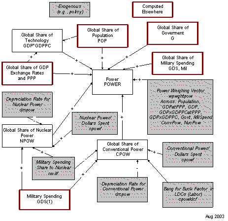
Conventional and nuclear power have their own dynamics, dependent primarily on military spending. Parameters direct a share of that into nuclear power and determine the translation of spending into actual conventional power, with an assumption that Less Developed Countries can leverage spending into more power because of lower wages and other costs. Given country/regional conventional and nuclear power, it is possible to compute world conventional and nuclear power (CPOW, NPOW).

Threat Level

The threat that any state poses to another (and which may lead to conflict, war, or nothing) is affected by many factors. IFs conceptualizes of threat in concrete terms, namely the probability of what is called a militarized international dispute (MID).

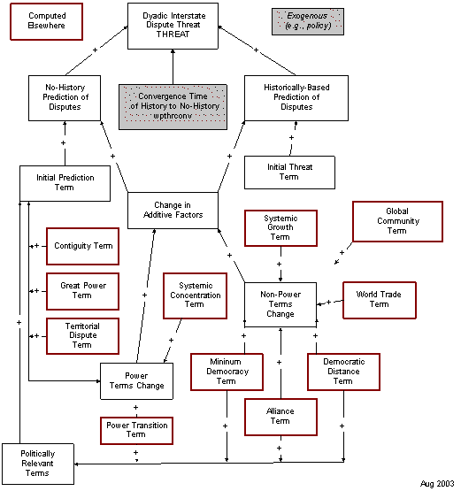
IFs approaches calculation of that threat from two directions. The first is through the use of data on historic threat levels by dyad. The second is solely through the evolution of key factors that have been shown to give rise to disputes. The user can control whether the model should rely primarily upon historic patterns or primarily upon predicted ones with a convergence parameter (wpthrconv).

Regardless of the basic approach (data-based or predictive), the evolution of threat over time depends upon a variety of underlying factors. IFs groups these roughly into two categories: power and nonpower terms, explained in detail elsewhere. It should be noted, however, that three factors seem to carry special weight in determining the threat of disputes: contiguity, whether or not countries are great powers, and the existence or absence of territorial disputes between countries.

Visual representation of threat level

Threat Elaborated: Power Terms

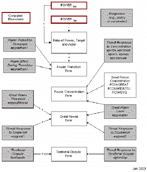
One important power term that affects interstate relations depends on relative power of the countries and is especially significant when two countries of relevance to each other enter a zone of power transition. Another important term is the concentration of power among the great powers themselves. It is increasingly uncertain whether the European Union should be treated as a single actor or as a group of individual states in such power concentration calculations, so IFs allows an option.

A third factor is whether or not the two interacting states are great powers or not. It is important whether the dyad contains zero, one, or two such powers. Because the definition of great power is uncertain, IFs allows the user to specify a threshold level at which a state begins to meet that definition and a second level at which point it clearly does.

A fourth factor in the figure below is less clearly a power term. Nonetheless, existence or absence of territorial disputes between states greatly affects the probability of a militarized dispute, quite possibly more than any other single factor.

Threat Elaborated: Nonpower Terms

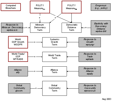
Among the most important factors that determine the probability of disputes between countries that are not related to their power is their level of democracy. More specifically, threat depends on the level of democracy in actor and target countries and on the difference in level, sometimes called political distance.

Studies find that trade relations between states also affect the probability of disputes between them, but results are ambiguous. Because IFs uses pooled trade, it cannot forecast the specific level of trade between any two states. The model has a term that links overall levels of global trade, as a portion of GDP, to dispute probability.

Alliances generally reduce dispute probability. Another factor that may reduce the probability is that global community is growing. This is uncertain and the linkage is not now activated.

One of the most basic factors affecting interstate relations is the closeness or contiguity of two states (small states on different continents pose little or no threat to each other).

Probability of War

The probability of conventional war depends most fundamentally on a basic conventional warfare probability per year (CWARBASE) that the user sets exogenously and that is set to zero for all country pairs (dyads) in the base case.

That probability is potentially enhanced by threat from an actor to a target country and also by the threat perceived by a target from an actor.

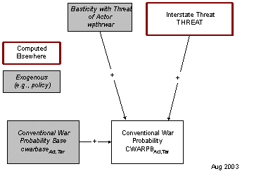
War

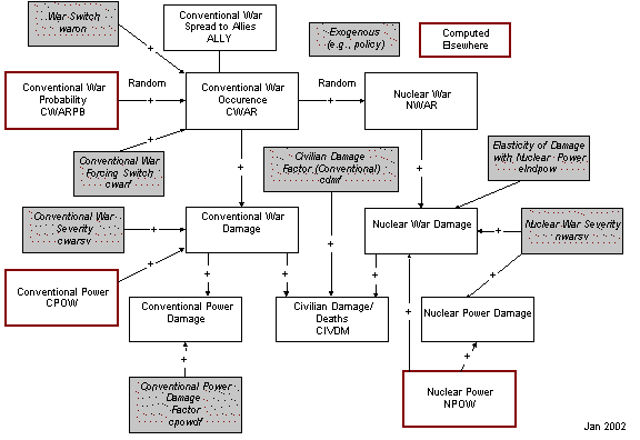
The outbreak of conventional war depends on the probability of war. The probability of war is converted into actual war randomly. The outbreak of nuclear war (only for countries with nuclear weapons) similarly depends probabilistically and randomly on the outbreak of conventional war. In order for a war to occur, the "waron" parameter must be turned on (set to 1). If it is turned on, wars may or may not occur; but a war can be forced if the waron parameter is set AND the war forcing switch (cwarf) is set to 100 or above).

We calculate damage for both conventional and nuclear power capabilities, as well as for civilian society (population and GDP).

IP6.gif

Interstate Politics Equations

For help understanding the equations see Notation.

IP Equations: Power

Foreign relations of states are sensitive to power calculations. There is a vast literature surrounding the measurement of power, with much debate among analysts around the components that should enter into calculations of power capabilities and how those components can best be aggregated into a single measure of power. Ray (1990) did a good job of reviewing that literature and has, himself, contributed to power calculation. Working with the Correlates of War project at the University of Michigan, he and others have frequently emphasized three primary components of power capabilities: economic, demographic, and military strength.

The early representation of power in IFs used a formulation that aggregated these three components and that further differentiated between conventional and nuclear military strength. It allowed the user to provide weightings for the three. For instance, many analysts are loath to weight demographic size heavily for less economically developed countries like India.

Over time, users of the model suggested that other components of power should also be considered. For instance, Evan Hillebrand suggested that economic-technological capability, as indicated by the product of GDP and GDP per capita, should be a core component of capabilities. There has also been a long tradition, dating at least to Ray Cline, suggesting that government capabilities (as perhaps indicated by government spending levels) should be an element. And there is uncertainty as to whether GDP is best measured for power purposes at purchasing power parity (PPP) or exchange rates. In response to these suggestions, it was decided to create a more general function for POWER in IFs that allows the user to create a flexibly weighted sum of 9 different components: population (POP), GDP at purchasing power (GDPP), GDP at market prices (GDP), economic-technological capability using GDP per capita at either purchasing power or exchange rates (GDPPCP, GDPPC), government size (GOVCON), military spending (GDS), conventional military power (CPOW) and nuclear power (NPOW). For each component, a global sum is created and country capabilities are computed as portions of the global total. Setting a weight to zero removes the component from the power calculation. In the base or default case, most or all weights (wpwghtpow) other than the ones on economic, demographic, technological, and military strength are set to zero.

$POWER_{\gamma }=AnalFunc(POP_{\gamma },GDPP_{\gamma },GDP_{\gamma },GDPPCP_{\gamma },GDPPC_{\gamma ,},GOVCON_{\gamma },GDS_{\gamma ,g-Mu},CPOW_{\gamma },NPOP_{\gamma },\mathbf {wpwghtpow_{pc}} )*100$

Conventional power (CPOW) for each entity decreases with depreciation (drcpow) and increases with the non-nuclear portion (1-nmilf) of annual military spending. A conventional power factor variable (CPowF) converts new military spending into conventional capability. That factor is computed so that the spending by countries with GDP per capita below $10,000, because such countries can hire personnel at lower cost, has additional leverage in creating conventional power, as determined by a developing country conventional power factor (cpowldcf). The additional leverage is phased out as GDP per capita increases. The calculation of nuclear power (for those states that spend some portion of their military on nuclear capabilities) is analogous, but conversion of spending to power depends on a factor (npowf) that is invariant across countries.

$CPOW_{\gamma }=CPOW_{\gamma }^{t-1}*(1-\mathbf {drcpow} )+GDS_{\gamma ,s=1}*(1-\mathbf {nmilf} _{\gamma })*CPowF_{\gamma }$

where

$CPowF_{\gamma }=\mathbf {cpowldcf} -(\mathbf {cpowldcf} -1)*{\frac {Min(10,GDPPC_{\gamma })}{10}}$

$NPOW_{\gamma }=NPOW_{\gamma }^{t-1}*(1-\mathbf {drnpow} )+GDS_{\gamma ,s=Mil}*\mathbf {nmilf} _{\gamma }*\mathbf {npowf} _{\gamma }$

As indicators, it is also useful to calculate the world total of conventional (WCPOW) and nuclear power (WNPOW).

$WCPOW=\sum ^{R}CPOW_{\gamma }$

$WNPOW=\sum ^{\gamma }NPOW_{\gamma }$

IP Equations: Overview of Threat Formulation

The threat that one country poses to others is a key concept in IFs. Unlike most variables in IFs, it is dyadic (actor country to target country). It is also different from most IFs variables in that it is a concept that has a probabilistic element in its implications for forward linkages. In fact, it is possible to think about threat as being the probability of military challenge or war, and that is the conceptualization in IFs. The database on Militarized Interstate Disputes (MIDS) was used in both conceptualization and initialization of threat in IFs.

Because of its importance, a substantial sub-project, sponsored by the Strategic Assessments Group (SAG) of the CIA devoted time to specifying the drivers of threat and the formulation for creating forecasts based on those drivers. Although none of the participants in that subproject bear ultimate responsibility for the treatment of threat in IFs, the model owes a substantial debt to the sponsors and participants of that sub-project.

Three key distinctions are important to understanding the overall threat formulation and its use in forecasting:

1. Using history to initialize threat levels versus using predictive formulations. The argument for using data to initialize dyadic threat levels is obvious: data tell us about historic relationships between countries like India and Pakistan, often carrying information that is not available in a predictive formulation calculated across many dyads and not picking up the historic path elements of a particular dyad. Yet the argument for not relying too heavily on such dyadic data in forecasting is also obvious: the U.S.-Russian relationship has fundamentally changed since the collapse of communism and the break-up of the Soviet Union, so that a forecast based heavily on historic data would now be questionable. The IFs formulation provides forecasts that are rooted in data, but it allows the user to relax the ties to historic data over time.
2. The complicated contribution of constant terms, switches, and variables. The single best predictor of conflict among countries historically may well be their physical proximity, with contiguous or geographically touching countries being much more conflict prone. But because contiguity is a constant, it is near useless in determining how the threat of overt conflict will change in the future. Somewhat similarly, territorial disputes are a near constant over time, but can be switched on or off. Quite differently, power levels and commitment to democracy fluctuate substantially over time. The different types of variables enter differently into the formulation.
3. The contribution of power-based drivers and other drivers. For purposes of clarity of conceptualization and presentation of it, there is value in distinguishing between drivers of threat that have their roots primarily in state power and those, like democracy level, that do not.

Taking into account these important distinctions, the IFs formulation of threat has three key components. The first is a constant base term rooted in data and/or predictive theory. When it is rooted in predictive theory, the term draws on the constant and switch inputs to threat such as contiguity and territorial dispute. When it is rooted in data it represents recent history for the dyad as computed by the MIDs data. The second term is a delta or variable term rooted in power variables and the third term is a delta term rooted in non-power variables. The model user can use a parameter (wpthrconv) to determine whether the ultimate threat calculation (THREAT) should remain tied to the empirical initial condition (THREATIDATA), as modified by the delta terms, or should converge over time to a fully predicted threat formulation (THREATIPRED), again modified by delta terms.

$THREAT_{act,ta{\gamma }}=ConvergeOverTime(ThreatData_{act,ta{\gamma }},ThreatPred_{act,ta{\gamma }},wpthrconv)$

where

$ThreatData_{act,ta{\gamma }}=ThreatIData_{act,ta{\gamma }}+DeltaPowerTerms+DeltaNonPowerterms$

$ThreatPred_{act,ta{\gamma }}=ThreatPred_{act,ta{\gamma }}+DeltaPowerTerms+DeltaNonPowerTerms$

It is useful also to be able to see a summary measure of the average world threat level (WTHREAT) over time. The sum of all threat terms is normalized by the product of the number of regions (NR) times the number – 1 (there are no non-zero and meaningful self-threat terms).

$WTHREAT={\frac {\sum ^{A}\sum ^{T}THREAT_{act,ta{\gamma }}}{NR*(NR-1)}}$

IP Equations: Threat Formulation Subproject

The Strategic Assessment Group (SAG) of the Central Intelligence Agency sponsored a sub-project of IFs with the title of Threats and Opportunities Analysis (TAOS). Guided by Evan Hillebrand from SAG, a number of experts were drawn together to review and discuss enhancements to the IFs system, notably its representation of interstate politics. The participants were Stuart Bremer, Mark Crescenzi, Doug Lemke, Edward Mansfield, and Paul Senese.

The project ultimately facilitated the incorporation into IFs of insights from these individuals as well as work recommended by them See Crescenzi and Enterline (2001), Huth (1996), Mansfield (1994), and Tammen, Kugler, Lemke, Stam, Alsharabati, Abdollahian, Efird, and Organski (2000). See, also, Bennett and Stam (2003), who were good enough to provide an early manuscript draft of their book.

In addition, the project was able to draw on the database for militarized interstate disputes (MIDs) involving “the threat, display, or use of military force short of war” (Jones, Bremer and Singer 1996: 163). At the time of analysis for IFs the MIDs database did not extend beyond 1992, however, complicating estimation for the post-Cold War period.

Some of the parameters for relationships in the IFs threat calculation were derived from Bennett and Stam. Senese estimated parameters for the democracy relationships from MIDs data. And Lemke put together a set of estimated and literature-based parameters that helps determine most of the base-case values in IFs. The parameter determination was guided by the desire to create a set of what economists sometimes call “stylized facts,” indicating the contribution of various factors to higher or lower probabilities of conflict in a dyad. For a detailed description of the work from that project and the formulation it produced, see Hughes, 2002.

IP Equations: Initial Threat Terms

Threat in a dyad is calculated using either empirically based initial conditions (ThreatIData) or predicted initial conditions (ThreatIPred). Empirical values come from the Militarized International Dispute (MIDs) database. Mark Crescenzi provided empirical initial conditions from that database using a technique for representing "memory" of past events (more distant events are less memorable) that he and Andrew Enterline pioneered (Crescenzi and Enterline 2001). A significant problem was that the initial conditions for dyads involving Cold War adversaries were no longer credible after the end of the Cold War. Moreover, the MIDs database used for the estimations extended only to 1992. Therefore the IFs project relied on expert judgment to reset some of those value: essentially, conflict for important Cold-War dyads like the U.S.-Russia was put at zero after 1992 and the Crescennzi-Enterline technique was used through 2002 in order to erode the earlier Cold-War memory in the creation of initial conditions.

Predicted initial conditions use a formulation that relies on some of the strongest empirical predictors of interstate conflict. The first three are constant or switch factors: great power status of the dyad members, contiguity, and existence of territorial dispute (all of which substantially increase the threat of conflict). Each term merits some comment:

• Great power status is often (for instance, in the Correlates of War project) determined subjectively. Because IFs needs to forecast that status, not just to apply it without change over time, the model needed an objective definition of it. In general it may be safe to argue that all states with more than about 5% of total systemic power are great powers, and no states with less than 2% of systemic power are great powers. Yet even those cut-offs could be debated. Because of the range of uncertainty, IFs uses a variable representation of the status, designating any state below the lower level (carried by the parameter wpgreatthesh) as a non-great power, and any state above the upper level (wpgreatlev) as a great power, conferring partial status in between for selected computations (like that of systemic power concentration). The internal IFs variable GPowerTermI carries the resulting calculation of increased threat of conflict from great power status in the dyad, where wpgreat1 determines the contribution of full great power status and wpgreat2 determines the contribution of partial great power status.
• Paul Diehl generously provided contiguity data for IFs (CONTIGUITY) and the parameter wpcontiguity translates the impact of contiguity into increased threat of conflict (ContiguityTerm).
• The work of Paul Huth (1996) was tapped for territorial disputes (TerDispute). The parameter wpterdisp translates the existence of a dispute into increased threat of conflict (TerDisputeTerm).

$ThreatIPredBase_{act,ta{\gamma }}=GPowerTermI_{act,ta{\gamma }}+ContiguityTermI_{act,ta{\gamma }}+TerDisputeTerm_{act,ta{\gamma }}$

where

$GPowerTermI_{act,ta{\gamma }}=AnalFunc(POWER_{act},POWER_{ta{\gamma }},\mathbf {wpgreatthresh,wpgreatlev} ,wpgreat1,wpgreat2)$

$ContiguityTermI_{act,ta{\gamma }}=Contiguity_{act,ta{\gamma }}*\mathbf {wpcontiguity}$

$TerDisputeTerm_{act,ta{\gamma }}=TerDispute_{act,ta{\gamma }}*\mathbf {wpterdisp}$

If any of these three factors are positive, the dyad members are "politically relevant" to each other, thereby increasing their sensitivity to other factors. In politically relevant dyads, IFs adds three other factors to the calculation of initial threat levels: a power transition term, an alliance term, and a two-term democracy representation. Again, each factor needs elaboration:

• The initial power transition term (PowerTranTermI) begins with a computation of the ratio of power within the dyad (PowerRatio). If that ratio exceeds a threshold level (wppowtran1) then the increased threat of conflict in the power transition term is set equal to the difference between the power ratio and the threshold power transition level, multiplied by an impact parameter (wppowtran2).
• The alliance term (AllyI) is simply the exogenously-specified existence (1) or absence (0) an alliance times a parameter (wpally) than translates alliance into conflict reduction.
• Senese has found that the impact of democracy on the threat of conflict depends on both the lesser level of democracy in the states of the dyad and the difference between their levels. The lesser or minimum level is multiplied by a parameter (wpdemmin) to determine the minimum democracy term (DemocTermMin) and the distance in democracy is multiplied by a second term (wpdemdist) to determine the contribution of the distance term to changed threat of conflict (DemocTermDist).

if $ThreatIPredBase_{act,tay}>0$

then $ThreatIPred_{act,ta{\gamma }}=ThreatIPredBase_{act,ta{\gamma }}+PowerTranTermI_{act,ta{\gamma }}+AllyI_{act,ta{\gamma }}+DemocTermMin_{act,ta{\gamma }}+DemocTermDist_{act,ta{\gamma }}$

where

$PowerTranTermI_{act,ta{\gamma }}=AnalFunc(POWER_{act},POWER_{ta{\gamma }},\mathbf {wppowtran1} ,\mathbf {wppowtran2} )$

$AllyI_{act,ta{\gamma }}=ALLY_{act,ta{\gamma }}*\mathbf {wpally}$

$DemocTermMin_{act,ta{\gamma }}=Amin(DEMOCPOLITY_{act},DEMOCPOLITY_{ta{\gamma }})*\mathbf {wpdemmin}$

$DemocTermDist_{act,ta{\gamma }}=(DEMOCPOLITY_{act}-DEMOCPOLITY_{ta{\gamma }})*\mathbf {wpdemdist}$

IP Equations: Power Term for Threat

The threat calculation builds on an initial, constant term plus a delta power term (that is, a change in power term) and a delta non-power term. This topic explains the power term. It is a sum of four other terms: delta great power term (DeltaGPowerTerm), delta power transition term (DeltaPowerTranTerm), delta territorial dispute term (DeltaTerDisputeTerm), and delta power concentration term (DeltaConcenTerm). See the Initial Threat Topic for a discussion of the foundational elements of the first three of these. The delta term for each is the foundational term in a future year minus the initial value of the term. The only new term in future years is the delta power concentration term (DeltaConcenTerm), explained below.

$DeltaPowerTerm_{act,ta{\gamma }}^{t}=DeltaGPowerTerm_{act,ta{\gamma }}^{t}+DeltaPowerTranTerm_{act,ta{\gamma }}^{t}+DeltaTerDisputeTerm_{act,ta{\gamma }}^{t}+DeltaConcenTerm_{act,ta{\gamma }}^{t}$

where

$DeltaGPowerTerm_{act,ta{\gamma }}^{t}=GPowerTerm_{act,ta{\gamma }}^{t}-GPowerTermI_{act,ta{\gamma }}^{t-1}$

$DeltaPowerTranTerm_{act,ta{\gamma }}^{t}=PowerTranTerm_{act,ta{\gamma }}^{t}-PowerTranTermI_{act,ta{\gamma }}^{t-1}$

$DeltaTerDisputeTerm_{act,ta{\gamma }}^{t}=TerDisputeTerm_{act,ta{\gamma }}^{t}-TerDisputeTermI_{act,ta{\gamma }}^{t-1}$

$DeltaConcenTerm_{act,ta{\gamma }}^{t}=ConcenChange*\mathbf {wpcon} +ConcenChange^{2}*\mathbf {wpconsq}$

where

$GPowerTerm_{act,ta{\gamma }}^{t}=f(POWER_{act}^{t},POWER_{ta{\gamma }}^{t},\mathbf {wpgreatthresh,wpgreatlev} ,wpgreat1,wpgreat2)$

$PowerTranTermI_{act,ta{\gamma }}^{t}=f(POWER_{act}^{t},POWER_{ta{\gamma }}^{t},\mathbf {wppowtran1,wppowtran2} )$

$TerDisputeTerm_{act,ta{\gamma }}^{t}=TerDispute_{act,ta{\gamma }}^{t}*\mathbf {wpterdisp}$

$ConcenChange=Max(\mathbf {wpconmin} ,Min(\mathbf {wpconmax} ,PCONGREAT^{t}))-Max(\mathbf {wpconmmin} ,Min(\mathbf {wpconmax} ,PCONGREAT^{t-1}))$

Power concentration is a concept focusing on the degree to which the power structure of the great powers (not all powers in the system) is heavily concentrated or not. The measure poses an alternative to the often less systematic estimation of whether a system is multipolar, bipolar, etc. (Singer, Bremer, and Stuckey 1972). IFs calculates systemic power concentration using the Ray and Singer (1973) calculation approach,

$PCONGREAT={\sqrt {\frac {SumSharesSq-{\frac {1}{SumGreat}}}{1-{\frac {1}{SumGreat}}}}}$

where

$SumSharesSq=\sum ^{GPowers}({\frac {POWER_{\gamma }}{\sum ^{GPOWERS}POWER_{\gamma }}})^{2}$

$SumGreat=NumberofGreatPowers$

More specifically, IFs calculates four versions of power concentration. The first (PCONGREAT) is the most traditional, using a fixed cut-off for defining great powers (wpgreatlev) and normally setting that value at 5%. The measure also treats all European Union members as individual countries. The second variation (PCONGREATEU) treats the European Union as a single entity. The user has a parameter (eumembsw) to define membership in the EU over time. Although few would argue that it currently acts as a single great power, greater unity is possible in the future. Both of the first two measures are, however, somewhat erratic in forecasts, because they make a fixed distinction about great power status at the threshold level. Thus if Japan drops below five percent of systemic power (as it normally does relatively early in the base case), the number of powers considered changes and there is a transient in the calculation of power concentration. Because that seems rather arbitrary, a third measure (PCONGREATF) uses a more flexible measure of great power, phasing the status in or out above a threshold (wpgreatthresh) up to full status (wpgreatlev). The fourth measure does the same for the single EU variant (PCONGREATEUF). For completeness, IFs also calculates a global concentration measure (PCONSYS), not distinguishing between great and other powers.

Edward Mansfield (1994) has investigated the relationship between power concentration of great powers and propensity for war in the system, finding a non-linear pattern with war most likely at highest and lowest system concentration levels. Bennett and Stam (2003) investigated the relationship for MIDs rather than wars, and found parameters about half the magnitude that Mansfield reported for wars. IFs uses a Mansfield-type non-linear formulation, with reduced parameters more appropriate to disputes rather than wars (remember that the IFs approach is a fundamentally stylized one, bringing together insights from much research rather than relying on a single analysis).

The Mansfield formulation looks to change in power concentration (ConcenChange) and to the square of change in power concentration for impact on the threat of conflict, which is the reason that power concentration enters only the delta term, not the initial term. Parameters on the change in power concentration (wpcon) and the square of the change (wpconsq) determine the ultimate concentration term. Also in the above calculation, power concentration is bound at all time points to be between a minimum (wpconmin) and maximum (wpconmax) value. Mansfield suggests that the analysis is only valid for values between .202 and .417.

IP Equations: Non Power Term for Threat

The threat calculation builds on an initial, constant term plus a delta power term (that is a change in power term) and a delta non-power term. This topic explains the non-power term (DeltaNonPowerTerm). It is a sum of five other terms: delta minimum democracy term (DeltaDemocTermMin), delta democracy distance term (DeltaDemocTermDist), delta alliance term (DeltaAllyTerm), delta trade term (DeltaTradeTerm), and delta GDP growth term (DeltaGDPGrowthTerm). See the Initial Threat Topic for a discussion of the foundational elements of the first three of these. The delta term for each is the foundational term in a future year minus the initial value of the term. The two new terms in future years are the delta trade term (DeltaTradeTerm) and delta GDP growth term (DeltaGDPGrowthTerm), both explained below.

$DeltaNonPowerTerm_{act,ta{\gamma }}^{t}=DeltaDemocTermMin_{act,ta{\gamma }}^{t}+DeltaDemocTermDist_{act,ta{\gamma }}^{t}+DeltaAllyTerm_{act,ta{\gamma }}^{t}+DeltaTradeTerm_{act,ta{\gamma }}^{t}+DeltaGDPGrowthTerm_{act,ta{\gamma }}^{t}$

where

$DeltaDemocTermMin_{act,ta{\gamma }}^{t}=GDemocTermMin_{act,ta{\gamma }}^{t}-GDemocTermMinI_{act,ta{\gamma }}^{t-1}$

$DeltaDemocTermDist_{act,ta{\gamma }}^{t}=DemocTermDist_{act,ta{\gamma }}^{t}-DemocTermDistI{t-1}_{act,ta{\gamma }}$

$DeltaAllyTerm_{act,ta{\gamma }}^{t}=AllyTerm_{act,ta{\gamma }}^{t}-AllyTermI_{act,ta{\gamma }}$

$DeltaTradeTerm_{act,ta{\gamma }}^{t}={\frac {WTRADE^{t}-WTRADE^{t-1}}{100}}*\mathbf {wptrade}$

$DeltaGDPGrowthTerm_{act,ta{\gamma }}^{t}={\frac {WGDPR^{t}-LongTermGDPR^{t}}{10}}*\mathbf {wpsysgr}$

where

$DemocTermMin_{act,ta{\gamma }}=Amin(DEMOCPOLITY_{act},DEMOCPOLITY_{ta{\gamma }})*\mathbf {wpdemmin}$

$DemocTermDist_{act,tay}=(DEMOCPOLITY_{act}-DEMOCPOLITY_{ta{\gamma }})*\mathbf {wpdemdist}$

$AllyI_{act,ta{\gamma }}=ALLY_{act,ta{\gamma }}*\mathbf {wpally}$

$LongTermGDPR^{t}=LongTermGDPR^{t-1}*.8+WGDPR^{t}*.2$

The preponderance of empirical analysis appears to support the proposition that trade relationships reduce conflict, contributing with joint democracy to enhanced peace among states in the manner that Kant posited long ago. Most of the studies focus on trade specific to the dyad, generally using dyadic trade over GDP as a measure of trade dependence, and often focusing on the less dependent of the two trading partners (Oneal and Russett 1997). Bennett and Stam (2001) support the general tendency of these conclusions (although Barbieri 1997 challenges them). IFs does not represent dyadic trade, but Mansfield (1994) found that systemic trade over GDP is also inversely related to war, at least for the great powers. IFs has such an inverse relationship with change in world trade as a percent of world GDP (WTRADE), controlling it by a parameter (wptrade) that is set rather low in the base case. In fact, because the parameter used was derived from dyadic analysis, IFs arbitrarily divides it by 10 in order to dilute the affect when using a global trade representation. Even then, this is a rather powerful factor, because the base case of IFs normally exhibits a continuation of the historic increase in global trade as a percent of GDP.

Bennett and Stam (2003) also investigated the impact of global economic cycles and found that conflict propensity of all kind roughly doubles during upswings relative to downswings. IFs introduces a factor that compares global economic growth (WGDPR) with the long term pattern (LongTermGDPR), computed as a moving average. IFs translates the swings of growth into impact on threat with a parameter (wpsysgr), once again looking to Bennett and Stam for guidance on the magnitude of it. The Bennett and Stam estimate, however, was remarkably high, higher than any other driver of conflict potential other than the addition of a second great power to the dyad. Because this seemed theoretically implausible, the base case normally uses a value that was arbitrarily reduced by about a factor of 5.

IP Equations: Action/Reaction

The model links the threat indicator to an action-reaction dynamic only if the model user leaves the action-reaction switch (ACTREAON) at "1." Setting it to 0.0 will turn off action-reaction. When that switch is thrown, threat affects military spending in a process that can set up a positive feedback loop to increase or decrease the spending of acting and reacting countries or regions. The model calculates a multiplier on military spending (GKMUL) based on the level of threat (THREAT) in comparison with the initial level. Dyads have different reactivities to each other; the United States is not as concerned by an increase in British defense spending as by an increase in Chinese spending – in fact the U.S. might welcome the British increase and feel able to shave its own rather than increase it. A parameter (reac) gives the user control over this reactivity differential. In the GLOBUS modeling project, Dale Smith developed a formulation to endogenize such reactivity coefficients for dyads, in response to trade and other factors. Because the dyadic threat formulation of IFs already incorporates a very large number of dyadic and global factors, it would be redundant to build them into the reactivity parameter, which serves, instead, to provide the user some dyadic specific control over arms spending action/reaction. The addition of the number 10 to numerator and denominator in the formulation has a fundamentally technical basis – if there is a very low level of initial threat in a dyad (say Belgium and Ecuador), small changes in the numerator should not be permitted to give rise to large changes in the ratio and therefore the multiplier on defense spending.

$GKMUL_{\gamma ,ta{\gamma }}={\frac {\sum ^{ACT}(THREAT_{act,ta}^{t}*\mathbf {reac} _{act,ta{\gamma }}+10)}{\sum ^{ACT}(THREAT_{act,ta}^{t-1}*\mathbf {reac} _{act,ta{\gamma }}+10)}}$

The multiplier shifts government expenditures into or away from the military and adjusts all other categories of expenditures proportionately to their size as calculated earlier, normalizing all expenditures (GDS) to the total level of government consumption (GOVCON).

$GDS_{\gamma ,s}=F(GDS_{\gamma ,S}^{*},GKMUL_{\gamma -ta{\gamma }},GOVCON_{\gamma })$

The action-reaction dynamic thus works across the entire governmental expenditure and economic model. For instance, the normal "burden" term in the action-reaction dynamic is unnecessary because the economic model captures the burden of increased government spending on the military when it reduces spending on health and education.

IP Equations: War

IFs conceptualizes the threat variable (THREAT) as a probability of conflict, and initial conditions and parameters for its calculation were estimated primarily from militarized interstate dispute data. Across all dyads only a small portion (wpthrwar) of militarized disputes result in actual war. Knowing that percentage, it is possible to translate THREAT into the actual probability of war (CWARB), a variable that ranges from 0 to 100 (100% being certainty), just as THREAT ranges from 0 to 100. To allow the user more complete control over the probability of war in any given dyad, a second parameter (cwarbase), with a default value of 0, can be set from 0 to 100. Obviously, many variables, including factors such as relative power, affect whether or not countries in a dyad go to war. Remember that the THREAT variable is calculated so as to be responsive to such factors.

$CWARPB_{act,ta{\gamma }}=THREAT_{act,ta{\gamma }}*\mathbf {wpthrwar+cwarbase} _{act,ta{\gamma }}$

Even after the calculation of a war probability, however, IFs does not automatically proceed to generate a war and compute its consequences. The main reason is that, in the process of translating a probability into an event using a random number generator, a randomness is introduced into any model doing so. The philosophy of IFs use is that, unless the user consciously adds a random element, any run with a given set of parameters should always generate the same results and thus be easily compared with the base case.

Thus proceeding from probabilities of war to actual war events requires action on the part of the model user. Specifically, turning on a war parameter (waron) by moving it from the default value of 0 to the on value of 1 will do engage the linkage from war probabilities to war events.

There are two additional parameters that give users further control over war, once the waron parameter is set to 1. First, the conventional war base parameter (cwarbase), as noted above, can be adjusted. A value of 100, when waron is set to 1, will force a war in a given dyad. Second, a conventional war parameter (cwarf), also normally set to 0, can be set to 100 or more to force wars in all dyads, a true global war. The purpose of doing so is to allow assessment of damage potential from war, not because it is expected that a truly all-world war would ever occur.

As indicated, a random number generation function (RNDF) controls the process of moving from probability of war to actual conventional war (CWAR=1) or lack of it (CWAR=0). When waron is set to 1, a dyad in which the probability of war were an unusually high 10 percent would experience a war approximately every 10 years. Still, random behavior can generate a war each year or no war over 100 years.

if $\mathbf {waron} =1$ then $CWAR_{act,ta{\gamma }}=RNDF(CWARPB_{act,ta{\gamma }})$

if $\mathbf {cwarf} >100$ then $CWAR_{act,ta{\gamma }}=1$

The length of any conventional war (LENWAR) is purely random and varies from 1 to 6 years.

When nuclear powers are involved in conventional war, there is always a possibility of the escalation to nuclear war (NWARPB). The probability depends on the existence of the conventional war, an exogenously specified severity of war (cwarsv), and an exogenously specified probability for escalation (nwarf). Again, a random number generator translates that probability into the existence (NWAR=1) or nonexistence (NWAR=0) of nuclear war.

$NWARPB_{act,ta{\gamma }}=CWAR_{act,ta{\gamma }}*\mathbf {cwarsv*nwarf}$

$NWAR_{act,ta{\gamma }}=RNDF(NWARPB_{act,ta{\gamma }})$

When war occurs, there are at least two kinds of consequences. The first is a spread to allies of the members of a dyad. The second is damage to populations and economies.

With respect to the spread of war, IFs makes the simplifying assumption that all allies of each partner as specified exogenously in the alliance parameter (ally) become involved in the conflict. This is not always true, but the model user can easily control it through the alliance parameter.

With respect to the calculation of damage, IFs computes civilian damage multipliers (CIVDM) for all participants. The basic assumption is that damage to an active participant, the actor, is directly proportional through a severity factor (cwarsv) to the conventional power (CPOW) of the opposing participant, the target), and inversely proportional to the GDP of the actor. A further parameter, the civilian damage multiplier factor (cdmf) allows more complete control over the damage assessment. If there is a nuclear war involved as well as a conventional one, nuclear damage (NuclDam) from all "war partners" (targets) is added to the conventional damage.

The resultant civilian damage multiplier is used in population and economic models to reduce population and economic capital, as described in the documentation of those models.

if $CAWR_{act,ta{\gamma }}=1$ then $CIVDM_{{\gamma }-act}=\sum ^{Targets}{\frac {CPOW_{{\gamma }-ta{\gamma }}*\mathbf {cwarsv} }{GDP_{{\gamma }-act}}}*\mathbf {cdmf} +\sum ^{Targets}NuclDam_{{\gamma }-ta{\gamma }}$

where

if $NWAR_{act,ta{\gamma }}=1$ then $NuclDam_{{\gamma }-ta{\gamma }}=1-{_{.5}}({\frac {NPOW_{{\gamma }-ta{\gamma }}*nwarsv}{1000}})^{elndpow}$

War also weakens conventional power, through use and through destruction. The conventional damage multiplier (CPowDM) is fundamentally analogous to the civilian damage multiplier, except that it does not involve the inverse relationship to GDP size. The multiplier revises the earlier calculation of conventional power as it is carried forward to the next time period.

$CPOW_{\gamma }^{t+1}=CPOW_{\gamma }^{*,t+1}*(1-CPOWDM_{\gamma })$

where

if $CWAR_{act,ta{\gamma }}=1$ then $CPowDM_{\gamma }=\sum ^{Targets}CPOW_{{\gamma }-ta{\gamma }}*\mathbf {cwarsv} +\sum ^{Targets}NuclDam_{{\gamma }-ta{\gamma }}$

else

$CPowDM_{\gamma }=0$

IFs assumes the reduction of nuclear power only in the case of nuclear war (an assumption, as Iraq can testify, that is not always valid). The reduction in each country's or region's nuclear power is proportional to their initial power level (in nuclear wars, almost all nuclear power would presumably be used).

if $NWAR_{{\alpha },ta{\gamma }}=1$ then $NPOW_{\gamma }^{t+1}=NPOW_{\gamma }^{*,t+1}-NPOW_{\gamma }^{t}*\mathbf {nwarsv}$