Health
The most recent and complete health model documentation is available on Pardee's website. Although the text in this interactive system is, for some IFs models, often significantly out of date, you may still find the basic description useful to you.
The IFs health model allows users to forecast age, sex, and country specific health outcomes related to 15 cause categories (see table) out to the year 2100. Based on previous work done by the World Health Organization’s (WHO) Global Burden of Disease (GBD) project[1 ], formulations based on three distal drivers – income, education, and technology – comprise the core of the IFs health model. However, the IFs model goes beyond the distal drivers, including both richer structural formulations and proximate health drivers (e.g. nutrition and environmental variables). Integration into the IFs system also allows us to incorporate forward linkages from health to other systems, such as the economic and population modules. Importantly, IFs provides the user the ability to vary model assumptions and create customized scenarios; as such, IFs is a tool exploring how policy choices might result in alternative health futures.
This documentation supplements the third volume of the PPHP series, “Improving Global Health,” (Hughes et al, 2011) by providing technical details of health model integration into the IFs system. It includes the specific equations used to forecast outcomes and drivers, relative risk values for proximate drivers, and data manipulations related to model initialization and projection. We intend the IFs model to be fully transparent to all users, and invite comments and questions at http://www.ifs.du.edu/contact/index.aspx.
Cause groups in IFs
Group I – Communicable, Maternal, Perinatal, and Nutritional Conditions
- Diarrheal diseases
- Malaria
- Respiratory infections
- HIV/AIDS
- Other Group I causes
Group II – Noncommunicable Diseases
- Malignant neoplasms
- Cardiovascular diseases
- Digestive diseases
- Chronic respiratory diseases
- Diabetes
- Mental health
- Other Group II causes
Group III – Injuries
- Road traffic accidents
- Other unintentional injuries
- Intentional injuries
Structure and Agent System: Health
System/Subsystem
|
Health
|
Organizing Structure
|
Hybrid structure using distal driver formulations supplemented by proximate drivers; integrated with larger IFs systems such as population and governance
|
Stocks
|
Population by age-sex; stunted population; HIV prevalence
|
Flows
|
Births, mortality and morbidity
|
Key Aggregate Relationships (illustrative, not comprehensive)
|
Distal driver formulations driven by income, education, and time as a proxy for technological advance Proximate driver formulations driven by various social patterns and behaviors
|
Key Agent-Class Behavior Relationships (illustrative, not comprehensive)
|
Behavior related to proximate drivers such as smoking, indoor solid fuel use, obesity
|
Dominant Relations: Health
Health forecasting systems typically can help us either (1) to understand better where patterns of human development appear to be taking us with respect to global health, giving attention to the distribution of disease burden and the patterns of change in it; or (2) to consider opportunities for intervention and achievement of alternative health futures, enhancing the foundation for decisions and actions that improve health.
Broad structural models (e.g., that of the Global Burden of Disease or GBD) assist in the first purpose by relating deep or distal development drivers to outcomes. More specialized structural formulations and the inclusion of proximate drivers open the door to the second, allowing for consideration of interventions in the pursuit of alternate health futures. A more hybrid and integrated model form like that of IFs can help with both purposes and provide a richer overall picture of alternative health futures.
The figure shows the general structure. Formulations based on distal drivers (the GBD methodology) sit at its core. There is no inherent reason, however, that income, education and time (the distal drivers of the GBD approach) should be equally capable of helping us forecast disease in each of the major categories (let alone each of the specific diseases) that the GBD models examine. For example, distal driver formulations tend to produce forecasts of constantly decreasing death rates. Yet we know, for instance, that smoking, obesity, road traffic accidents, and their related toll on health tend to increase in developing societies among those who first obtain higher levels of income and education; with further societal spread of income and education, at least smoking and road traffic deaths (and perhaps also obesity) typically decline.[1 ]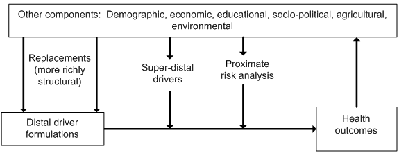
The integrated nature of the IFs modeling system further allows us to think about feedback loops between health outcomes and larger development variables such as economic progress and population structure.
[1] It is partly for this reason that the creators of the GBD models added exogenous specification of smoking impact to the otherwise mostly monotonically (one-direction only) changing specifications.
Health Flow Charts
Overview
Mortality from most causes of death is a function of a small number of distal or deep drivers and a larger number of proximate or more immediate drivers. For two specific mortality types, however, specifically deaths from AIDS and vehicle accidents, there are more specialized representations that rely on a number of more cause-related drivers.
Distal Drivers and Basic Indicators
To forecast mortality related to most of the major cause clusters we use the regression models and associated beta coefficients prepared for the GBD project (Mathers and Loncar 2006). Age, sex, cause, and country-specific mortality rate is a function of income (using GDP per capita as a proxy), adult education, technological progress. For specific death causes, smoking impact (for malignant neoplasms, cardiovascul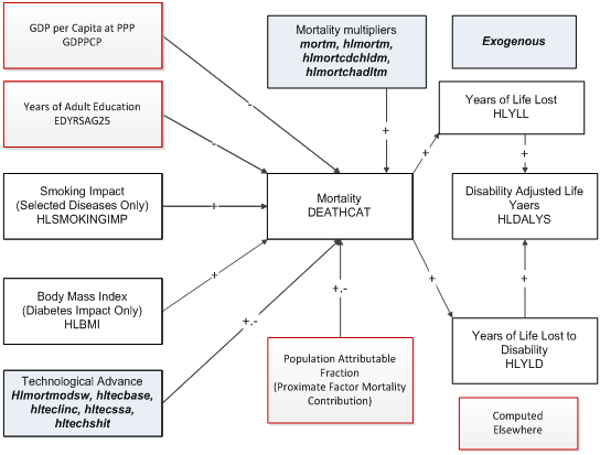
A number of parameters control technology in the distal functions. In the default mode (hlmortmodsw = 1), IFs modifies the technology (time) coefficient in recognition of slower than expected historical progress in many countries, an approach developed in the Global Burden of Disease (GBD project). Those country differences are controlled by hltechbase ,hltechlinc, and hltechssa. Setting the switch value to 0 activates an alternative IFs project approach to the impact of those parameters.
The user can also affect the mortality patterns directly with several parameters, including mortm , which allows simultaneous manipulation of all causes of death and hlmortm , which facilitates manipulation of each cause of death separately. Hlmortcdchldm changes the rates of all communicable diseases for children aged 5 and younger, while hlmortcdadltm affects rates of death from communicable diseases for adults aged 15-49.
Based on the mortality level, it is possible to compute the years of life lost to each cause of death (HLYLL). Using WHO-based estimates, IFs links mortality also to years of living with disability (HLYLD). The sum of the two is disability-adjusted life years lost (HLDALYS).
The forecast of mortality in this figure, dependent almost entirely on distal factors, is not actually the final calculation in the model. See the discussion of the entry of proximate drivers into the discussion of population attributable mortality fractions (PAFs), in interaction with distal-based mortality, for the rest of the story.
Because of the importance of smoking impact in the distal driver formulation, it is important that we elaborate that term. Body mass index is, at this point, only linked to diabetes and we discuss that in the context of the PAFs.
Smoking and Smoking Impact
Of the various specific health risks that the model treats, smoking has a special place because its impact is in the distal driver formulation of the IFs health model. The figure shows that the impact is driven by the rate of smoking (differentiated by males and females) 25 years earlier, with the relationship controlled by an impact elasticity (hlsmkel ). The user can also posit as a nearer term (in the model immediate) impact by setting a switch for that (hlsmkimeff ) at some fractional value of the full delayed impact–the value in the base case is 0.1 or 10 percent. For analysis purposes, another switch (hlsmimpsw ) can turn off the endogenous computation of smoking impact and leave it constant at the initial year value.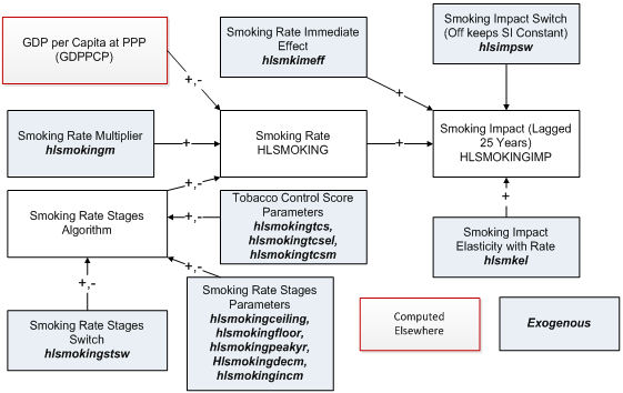
Smoking rate itself is computed in two different ways. The basic formulation uses only the initial condition and a function linked to the simple and squared values of GDP per capita at PPP. The more extended formulation is an algorithmic one based on the same general concept of a pattern that initially rises with GDP per capita, peaks, and then falls, but with a series of parameters that allow much more control over the stages.[1 ] This staged algorithmic approach (see Lopez et al. 1994; Shibuya et al. 2005; Ploeg et al. 2009) is turned on with a switch (hlsmokingstsw ).
Because control of tobacco is a major policy objective in many countries, there is also a representation of a tobacco control score on a 100-point scale (hlsmokingtcs ) with an associated parameter to control the elasticity of smoking with that score (hlsmokingtcsel ), as well as a multiplier on the score (hlsmokingtcsm ).
Finally, there is a multiplier that allows direct manipulation of the smoking rate, again by sex (hlsmokingm ).
[1] Cecilia Peterson developed this approach for IFs.Proximate Drivers and Risk-Specific Population Attributable Fractions
Overview
Although mortality can be calculated solely from distal drivers such as income and education, it is better to calculate it from proximate or more immediate factors, such as undernutrition or exposure to pollutants. But IFs, and perhaps any model, will never be able to represent all such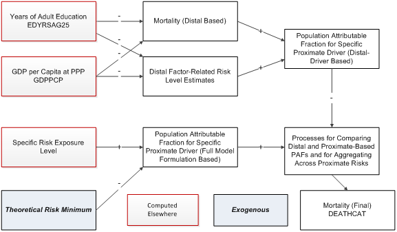
The figure below shows such a combination. Each proximate driver (and there are many different ones in IFs, in spite of the generalized representation in the figure) can be associated with a fraction of the mortality of a society. That population attributable fraction or PAF (derivative from the risk exposure level relative to a theoretical risk minimum) can be used to adjust the mortality associated with any cause that would have an implicit risk-related mortality built into the distal driver formulation. IFs makes those implicit distal-driver associated risk levels explicit by using the distal drivers to identify a risk level that would be expected based on cross-sectional analysis using the distal drivers. That allows the computation of a distal-driver based PAF. In similar fashion a PAF can be calculated that relates an exposure level to the risk, calculated mostly elsewhere in IFs (such as in the food and agriculture model for undernutrition of children) to a PAF.
The complication mathematically lies in the interaction of (1) the distal-driver and proximate risk-based PAFs and (2) the multiple specific-risk PAFs, because avoidance of death from one will generally increase the risk of death from others. See the equations associated with PAFs for details.
Among the specific risk factors treated in IFs are overly high body mass indices and associated obesity, undernutrition of children, access to unsafe water and sanitation, indoor use of solid fuels, and levels or urban air particulates.
Child Undernutrition
Although obesity is a growing problem and killer around the world, the most important risk factor for children in particular has traditionally been undernutrition (often simply referred to as malnutrition). The percentage of children undernourished (MALNCHP) affects mortality rates fr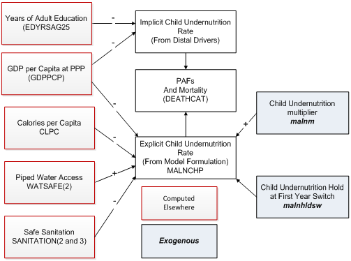
The figure below shows the approach for childhood undernutrition. The two key variables in the distal driver formulation at any point in time (ignoring the technology factor that adds dynamics over time) are GDP per capita at purchasing power parity and years of adult education. They are used in a cross-sectionally estimated function to calculate an implicit body mass index that then produces the associated implicit PAF. IFs uses an alternative and more risk-factor specific formulation to forecast values of child undernutrition over time. The PAF associated with this explicit representation of MALNCHP is compared with the PAF from the implicit calculation and the comparison alters the actual mortality pattern.
To calculate MALNCHP the explicit formulation also uses GDP per capita, as in the distal formulation, but augments it with calories per capita and with access to safe water and sanitation (unsafe water can cause diarrheal disease and undernutrition even with caloric intake would be adequate). A multiplicative parameter (malnchpm ) can be used to change child undernutrition in scenario analysis. Another parameter (malnchpsw ) can be used to hold the level of undernutrition at the level of the first year, an approach useful for counterfactual scenario analysis.
Although not used in the health model, IFs contains two other measure of undernutrition. The first is an alternative measure of child undernutrition developed by Smith and Haddad (2000); MALNCHPSH is computed as a function of the ratio of female and male life expectancy, of female secondary school gross enrolment rate, and of access to safe water. The second is a measure of rate of undernutrition for the entire population (MALNPOPP), computed as a function only of calories per capita.
Body Mass Index and Obesity
The distal driver formulation used for forecasting mortality in IFs contains a country’s average body mass index (HLBMI) for diabetes. HLBMI also affects mortality from cardiovascular disease in IFs via the mechanism that the model uses to modify cause-specific mortality from the distal driver formulation by actual risk level in a country. The core of that approach is to compare the risk-specific population attributable fraction (PAF) of total morality as calculated from the distal drivers with the PAF calculated from the actual level of the risk in the country.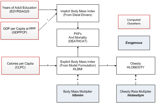
The figure below shows the approach for body mass index. The two key variables in the distal driver formulation at any point in time (ignoring the technology factor that adds dynamics over time) are GDP per capita at purchasing power parity and years of adult education. They are used in a cross-sectionally estimated function to calculate an implicit body mass index that then produces the associated implicit PAF. IFs uses an alternative and more risk-factor specific formulation to forecast values of body mass index over time. The PAF associated with this explicit representation of HLBMI is compared with the PAF from the implicit calculation and the comparison alters the actual mortality pattern.
To calculate HLBMI the explicit formulation uses calories per capita as the sole driving variable. A multiplicative parameter (hlbmim ) can be used to change HLBMI in scenario analysis. A forecast of the obese population as a percent of the total population (HLOBESITY) is driven by the body mass index. A separate multiplicative parameter can modify it (hlobesitym ).
Indoor Use of Solid Fuels
One of the most important health risk factors in the developing world, especially for women and children under 5 is the use of solid fuels for cooking (and heating) indoors (ENSOLFUEL). It is a major cause of respiratory diseases. In IFs it affects mortality rates via the mechanism that the model uses to modify cause-specific mortality from the distal driver formulation by using information concerning actual risk level in a country. The core of that approach is to compare the risk-specific population attributable fraction (PAF) of total morality as calculated from the distal drivers with the PAF calculated from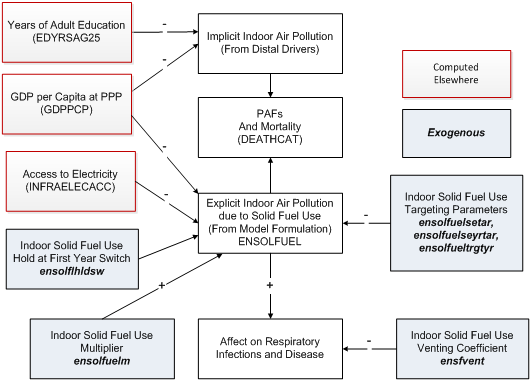
The figure below shows the approach for indoor air pollution from the use of solid fuels. The two key variables in the distal driver formulation at any point in time (ignoring the technology factor that adds dynamics over time) are GDP per capita at purchasing power parity and years of adult education. They are used in a cross-sectionally estimated function to calculate indoor air pollution (linked to solid fuel use) that then produces the associated implicit PAF. IFs uses an alternative and more risk-factor specific formulation to forecast values of solid fuel use over time. The PAF associated with this explicit representation of ENSOLFUEL is compared with the PAF from the implicit calculation and the comparison alters the actual mortality pattern.
To calculate ENSOLFUEL the explicit formulation also uses GDP per capita, as in the distal formulation, but augments it with access to electricity. For the actual equation, see the topic on equations for solid fuel use in the infrastructure documentation. A multiplicative parameter (ensolfuelm ) can be used to change solid fuel use in scenario analysis. Another parameter (ensolhldsw ) can be used to hold the rate of solid fuel use at the level of the first year, an approach useful for counterfactual scenario analysis.
Major factors affecting the health impact of indoor solid fuel use are the efficiency and ventilation of the stoves. The model provides a coefficient (ensfvent ) for scenario analysis concerning those factors.
Much analysis on this health issue will want to use control of solid fuel use, partly through the use of a multiplier (ensolfuelm ). There is also targeting of solid fuel use and the model provides two different kinds of targeting parameters, absolute and relative. The absolute (or universal) targeting allows the setting of a year (ensolfueltrgtyr ) by which solid fuel use would be eliminated; it is available country by country. The relative targeting approach, available only globally across all countries, allows the setting of a value based on the typical rate of solid fuel use at different levels of GDP per capita (estimated cross-sectionally). A target rate (ensolfuelsetar ) would normally be no higher than the typical rate at the country’s level of GDP per capita and could be, for instance, one standard error lower than the typical rate. An associated parameter (ensolfuelseyrtar ) identifies the number of years over which a country would move to the target level. If a country already meets or exceeds a relative target, it will not move (adversely) toward it. Moreover, only the absolute or relative target should be used in analysis, not both together–an attempt to use both together will result in neither being used.
Outdoor Urban Air Pollution
One of the more important health risk factors in the developing and developed world alike, especially for middle-income industrializing countries, is the concentration of particulate matter of diameter 2.5 micrometers or less per cubic centimeter in urban air (ENVPM2PT5).[1 ] It is a major cause of respiratory infections, respiratory diseases, and cardiovascular disease in adults 30 and older. In IFs it affects mortality rates via the mechanism that the model uses to modify cause-specific mortality from the distal driver formulation by using information concerning actual risk level in a country. The core of that approach is to compare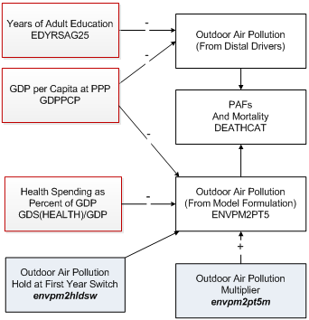
The figure below shows the approach for outdoor urban air pollution, focusing on the measure of ENVPM2PT5. The two key variables in the distal driver formulation at any point in time (ignoring the technology factor that adds dynamics over time) are GDP per capita at purchasing power parity and years of adult education. They are used in a cross-sectionally estimated function to calculate outdoor air pollution that then produces the associated implicit PAF. IFs uses an alternative and more risk-factor specific formulation to forecast values of outdoor urban air pollution use over time. The PAF associated with this explicit representation of ENVPM2PT5 is compared with the PAF from the implicit calculation and the comparison alters the actual mortality pattern.
To calculate ENVPM2PT5 the explicit formulation also uses GDP per capita, as in the distal formulation, but augments the spending of a country on health as a portion of GDP (which appears to serve reasonably well as a proxy for more general attention to the environment). For the actual equation, see the topic on outdoor urban air pollution equations in the health documentation . A multiplicative parameter (envpm2pt5m ) can be used to change urban air pollution in scenario analysis. Another parameter (envpm2hldsw ) can be used to hold the level of urban air pollution at the level of the first year, an approach useful for counterfactual scenario analysis.
[1] Initialized in IFs by converting World Bank data on PM10 concentrations.
Water and Sanitation
Although unsafe water and sanitation is a killer via its contribution to undernutrition of children in particular, it creates its own mortality risk especially via diarrheal disease. The variables of importance in IFs are access to safe water (WATSAFE) and safe sanitation (SANITATION). In IFs they affect mortality rates via the mechanism that the model uses to modify cause-specific mortality from the distal driver formulation by using information concerning actual risk level in a country. The core of that approach is to compare the risk-specific population attributable fraction (PAF) of total morality as calculated from the distal drivers with the PAF calculated from the actual level of the risk in the country.
The figure below shows the approach for safe water and sanitation. The two key variables in the distal driver formulation at any point in time (ignoring the technology factor that adds dynamics over time) are GDP per capita at purchasing power parity and years of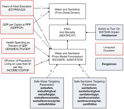
To calculate WATSAFE and SANITATION (separately) the explicit formulation also uses both average years of adult education and GDP per capita, as in the distal formulation, but augments those with the spending of a country on health as a portion of GDP (which appears to serve reasonably well as a proxy for more general attention to the environment) and portion of the citizenry living on less than $1.25 per day. For the actual equations, see the topic on outdoor urban air pollution equations in the infrastructure documentation.
Both access to safe water and to safe sanitation have ladders of access quality ranging from none to household connections. Parameters affecting them must thus take into account those ladders and the specific level(s) the parameter affects. Multiplicative parameters (watsafem and sanitationm ) can be used to change access at any level on the two ladders (the model normalizes access across levels to assure summation to 100 percent. Another parameter pair (watsafehldsw andsanithldsw ) can be used to hold the level of access at that of the first year, an approach useful for counterfactual scenario analysis.
Other parameters control targeting, both universal and relative. With respect to absolute targeting, watsafetrgtval and watersafetrgtyr control those with no access to safe water (the proportion and the number of years to reach the target, respectively). Similarly, sanitationtrgtval and sanitationtrgtyr control those with access to household connections. The relative targeting approach, available only globally across all countries, allows the setting of a value based on the typical rate of access at different levels of GDP per capita (estimated cross-sectionally). A target level (watsafenoconsetar, sanithhconsetar, sanitnoconsetar ) would normally be no better (which could mean no higher or no lower) than the typical level at the country’s level of GDP per capita and could be, for instance, one standard error better (higher or lower depending on the variable being targeted) than the typical level. An associated parameter (watsafenoconseyrtar, sanithhconseyrtar, sanitnoconseyrtar ) identifies the number of years over which a country would move to the target level. If a country already meets or exceeds a relative target, it will not move (adversely) toward it. Only the absolute or relative target should be used in analysis, not both together–an attempt to use both together will result in neither being used.
Specialized Models: Deaths from AIDS and Vehicle Accidents
AIDS deaths depend very directly on the number (or stock) of HIV-infected individuals, which depends in turn on the HIV-infection rate (HIVRATE). Data on HIV infection rates were used to compute a basic, country/region-specific rate of HIV infection increase (hivincrate), which the user can alter, as they can exogenous assumptions about the peak year of the epidemic (hivpeakyr) and the infection rate in that year (hivpeakr). If a country is beyond the peak year of the epidemic, control will be bringing the rate down over time (HIVTECCNTL). The user may also rely upon a country/region-specific multiplier to move rates up or down (hivm).
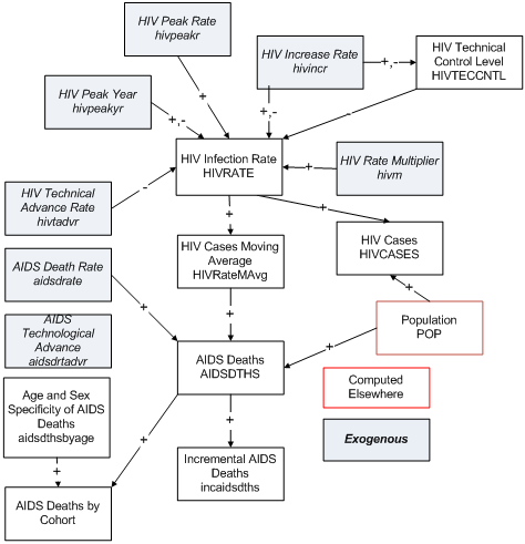
There is both a policy and medical effort underway to reduce the growth in infections. An HIV technical advance rate (hivtadvr) represents the success of that in rate of reduction in annual infection growth, and a variable (HIVTECCNTL) shows the cumulative impact of changes past a peak rate and year. Although highly speculative, the user will recognize the long-term importance of such assumptions.
Turning from the infection rate to the death rate, the user can make changes in the initial AIDS death rate (aidsdrate) to reflect possible progress or lack of it in reducing the deaths from HIV (using aidsdrtadvr). When the deaths from AIDS are computed, they are used to compute an incremental number of deaths (since some are already in the mortality of the base year); and an exogenous vector spreads them by age and sex.
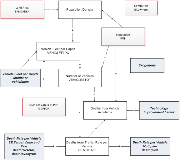
The computation of deaths from vehicle accidents starts with computing the number of vehicles per capita (VEHICFLPC) as a function of population density and GDP per capita. That allows computation of the total number of vehicles (VEHICLESTOT). The function used by IFs to compute the total number of road deaths uses th
Forward Linkages from Health
Overview
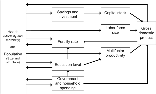
Chapter 7 of Hughes, Kuhn, Peterson, Rothman, and Solorzano (2011) elaborated the forward linkages of the health model to other parts of the IFs system at the time of that volume's completion. It begins by discussing a controversy in the literature about whether the effects on economic well-being (as indicated by GDP per capita) of improvements in life expectancy are positive or negative. It goes on to devote much attention to three major and general pathways of impact between health and GDP, each of which corresponds to an element in standard production functions and that in IFs. The diagram below shows the major pathways between health/demography and GDP, each of which requires elaboration by showing the variables and logic of the IFs system; those three are labor, capital, and multifactor productivity.
Forward Linkages of Health to Population and Labor Supply
The IFs demographic model captures the mechanical or accounting effects of mortality on population (see the solid paths in the figure below). A key pathway passes from mortality through adult age population to labor supply (including aging-related lags).[1] Similarly, IFs captures the mechanical effect of mortality on fertility through the death of women of childbearing age.
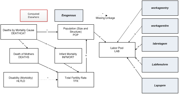
The most important non-mechanical linkage is almost certainly the relationship between child mortality and fertility. IFs forecasts fertility as a relationship with infant mortality, the log of educational level of those aged 15 and older (neither the education of women alone nor the education of those 15-24 work as well), and the percentage use of modern contraception.
[1] IFs also includes income-based formulations for changing the female participation rate.
Forward Linkages of Health to Capital Stock
</hgroup></header> The figure below sketches the primary paths between health (morbidity and mortality) and capital stock. Most capital stock consists of buildings and machinery for producing goods and services; some representations may include land also, but most treat land separately and largely as a constant (although land developed for crop production or grazing can, in fact, be highly variable, as it is in the IFs agricultural model). Most immediately, investment increases capital stock and depreciation reduces it. Although there is certainly some impact of morbidity and mortality on the rate of depreciation of both built physical and natural capital, the relationship may not be substantial and we do not understand it well enough to model it. Investment is responsive to both domestic savings and foreign flows.
Turning our gaze to the paths by which health affects investment, the three major ones run though health spending, which can crowd out savings and investment, through the age-structure of societies, which affects the savings rate, and through investment from abroad, which can augment that generated domestically.
With respect to health spending, to which we return later, the IFs model uses a social accounting matrix (SAM) structure. Thus the flow of funds into health spending automatically competes with other consumption uses and with savings and investment. The major current weakness of the model with respect to this path is that there is no linkage from morbidity (associated in IFs with mortality) and health expenditures. (There is a linkage in IFs back from health spending to mortality –all categories except for AIDS).
The paths in IFs that link age structure most directly to domestic savings have two important elements. The most fundamental one represents the understanding of life-cycle dynamics in income, consumption and savings. The cycle for income is fairly clear-cut with a peak in the middle to latter periods of the working years. Workers set aside some portion of income as savings and that portion, too, tends to peak in the middle and late period of working years. Society-wide savings themselves become negative after retirement age (65 in the Base Case scenario but variable in scenarios) even though some portion of the population will continue to work. The second fundamental element is that both the horizon of life expectancy and the average income level of a society can have an impact on the portion set aside for savings and the degree to which it rises and then falls. Thus, for example, the life-cycle “bulge” of savings may be earlier and flatter in developing countries.
We implemented the representation of savings and investment in accord with that understanding. Relying upon analyses of selected countries that Fernández-Villaverde and Kruegger (2004 and 2005) and Deaton and Paxson (2000) undertook, we extracted general stylized patterns of the savings life cycle to represent more and less developed (and lower life expectancy) countries. In forecasting we use the pattern for less developed countries when life expectancy falls below 40 years, use that for more developed countries when life expectancy exceeds 80 years, and interpolate in between for all other countries. The result of this largely algorithmic approach[1 ] is an adjustment factor (SavingsAgeAdj) that augments or reduces investment.
In addition, investment is somewhat augmented or reduced as a direct result of changing life expectancy. Life expectancy is compared over time with an expected value (tied to cross-sectional estimation with income). That difference is compared to the difference in the initial year and, if it rises, augments investment.
Although conceptually tied to savings rates, neither the life-cycle analysis nor the life-expectancy term directly affect savings in IFs. Instead, they affect investment directly and savings indirectly via the dynamics in IFs that balance savings and investment over time.
The path linking health to foreign direct investment is potentially quite important. Alsan, Bloom and Canning (2006: 613) reported that one additional year of life expectancy boosts FDI inflows by 9 percent, controlling for other variables. We have implemented that relationship in IFs. The representation of FDI in IFs captures the accumulation over time of FDI inflows in stocks of FDI, as well as the accumulation of FDI outflows in stocks. In addition, the stocks set up their own dynamics, including the tendency for stocks to reinforce flows. For that reason, we have set the base case parameter for the impact of each year of life expectancy on FDI flows to 0.05 (5 percent), lower than the estimate of Alsan, Bloom and Canning (2006).
[1] See the subroutine SavingsDemogAdj in routine Populat.bas, which draws upon table IncConSav in IFs.mdb with different patterns of income, consumption, and savings for more developed countries (MDCs) and less developed countries (LDCs) across age categories; in general, peaks of income, consumption, savings occur the in late 40s and savings turn negative at 65.