Education

Overview

The most recent and complete education model documentation is available on Pardee's website. Although the text in this interactive system is, for some IFs models, often significantly out of date, you may still find the basic description useful to you.

The education model of IFs simulates patterns of educational participation and attainment in 186 countries over a long time horizon under alternative assumptions about uncertainties and interventions (Irfan 2008).  Its purpose is to serve as a generalized thinking and analysis tool for educational futures within a broader human development context. 

The model forecasts gender- and country-specific access, participation and progression rates at levels of formal education starting from elementary through lower and upper secondary to tertiary. The model also forecasts costs and public spending by level of education. Dropout, completion and transition to the next level of schooling are all mapped onto corresponding age cohorts thus allowing the model to forecast educational attainment for the entire population at any point in time within the forecast horizon.

From simple accounting of the grade progressions to complex budget balancing and budget impact algorithm, the model draws upon the extant understanding and standards (e.g., UNESCO's ISCED classification explained later) about national systems of education around the world. One difference between other attempts at forecasting educational participation and attainment (e.g, McMahon 1999; Bruns, Mingat and Rakotomalala 2003; Wils and O’Connor 2003; Delamonica, Mehrotra and Vandemoortele. 2001; Cuaresma and Lutz 2007) and our forecasting, is the embedding of education within an integrated model in which demographic and economic variables interact with education, in both directions, as the model runs. 

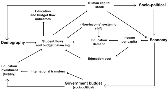
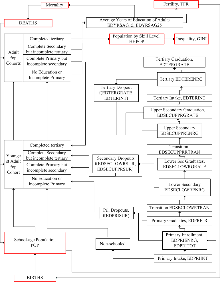
In the figure below we display the major variables and components that directly determine education demand, supply, and flows in the IFs system.  We emphasize again the inter-connectedness of the components and their relationship to the broader human development system.  For example, during each year of simulation, the IFs cohort-specific demographic model provides the school age population to the education model.  In turn, the education model feeds its calculations of education attainment to the population model’s determination of women’s fertility.  Similarly, the broader economic and socio-political systems provide funding for education, and levels of educational attainment affect economic productivity and growth, and therefore also education spending.

EduOverview.png

Structure and Agent System: Education

System/Subsystem	National Education System
Organizing Structure	Various Levels of Education; Age Cohorts
Stocks	Educational Attainment; Enrollment
Flows	Intake; Graduation; Transition; Spending
Key Aggregate  Relationships  (illustrative, not comprehensive)	Demand for and achievement in education changes with income, societal change   Public spending available for education rises with income level   Cost of schooling rises with income level   Lack (surplus) of public spending in education hurts (helps) educational access and progression   More education helps economic growth and reduces fertility
Key Agent-Class Behavior  Relationships (illustrative, not comprehensive)	Families send children to school; Government revenue and expenditure in education

Education Model Coverage

UNESCO has developed a standard classification system for national education systems called International Standard Classification of Education, ISCED. ISCED 1997 uses a numbering system to identify the sequential levels of educational systems—namely, pre-primary, primary, lower secondary, upper secondary, post-secondary non tertiary and tertiary—which are characterized by curricula of increasing difficulty and specialization as the students move up the levels. IFs education model covers  primary (ISCED level 1), lower secondary (ISCED level 2), upper secondary (ISCED level 3), and tertiary education (ISCED levels 5A, 5B and 6).

The model covers 186 countries that can be grouped into any number of flexible country groupings, e.g., UNESCO regions, like any other sub-module of IFs. Country specific entrance age and school-cycle length data are collected and used in IFs to represent national education systems as closely as possible. For all of these levels, IFs forecast variables representing student flow rates, e.g., intake, persistence, completion and graduation, and stocks, e.g., enrolment, with the girls and the boys handled separately within each country.

One important distinction among the flow rates is a gross rate versus a net rate for the same flow. Gross rates include all pupils whereas net rates include pupils who enter the school at the right age, given the statutory entrance age in the country and proceed without any repetition. The IFs education model forecasts both net and gross rates for primary education. For other levels we forecast gross rates only. It would be useful to look at the net rates at least for lower secondary, as the catch up continues up to that level. However, we could not obtain net rate data for lower secondary. 

Additionally, for lower and upper secondary, the IFs model covers both general and vocational curriculum and forecasts the vocational share of total enrolment, EDSECLOWRVOC (for lower secondary) and EDSECUPPRVOC (for upper secondary). Like all other participation variables, these two are also disaggregated by gender.

The output of the national education system, i.e., school completion and partial completion of the young people, is added to the educational attainment of the adults in the population. IFs forecasts four categories of attainment - portion with no education, completed primary education, completed secondary education and completed tertiary education - separately for men and women above fifteen years of age by five year cohorts as well as an aggregate over all adult cohorts. Model software contains so-called "Education Pyramid" or a display of educational attainments mapped over five year age cohorts as is usually done for population pyramids.

Another aggregate measure of educational attainment that we forecast is the average years of education of the adults. We have several measures, EDYEARSAG15, average years of education for all adults aged 15 and above, EDYRSAG25, average years of education for those 25 and older, EDYRSAG15TO24, average years of education for the youngest of the adults aged between fifteen years to twenty four.

IFs education model also covers financing of education. The model forecast per student public expenditure as a share of per capita income. The model also forecast total public spending in education and the share of that spending that goes to each level of education.

What the Model Does Not Cover

ISCED level 0, pre-primary, and level 4, post-secondary pre tertiary, are not common across all countries and are thus excluded from IFs education model.

On the financing side, the model does not include private spending in education, a significant share of spending especially for tertiary education in many countries and even for secondary education in some countries. Scarcity of good data and lack of any pattern in the historical unfolding precludes modelling private spending in education.

Quality of national education system can also vary across countries and over time. The IFs education model does not forecast any explicit indicator of education quality. However, the survival and graduation rates that the model forecasts for all levels of education are implicit indicators of system quality.  At this point IFs does not forecast any indicator of cognitive quality of learners. However, the IFs database does have data on cognitive quality.

The IFs education model does not cover private spending in education.

Sources of Education Data

UNESCO is the UN agency charged with collecting and maintaining education-related data from across the world. UNICEF collects some education data through their MICS survey. USAID also collects education data as a part of its Demographic and Household Surveys (DHS). OECD collects better data especially on tertiary education for its members as well as few other countries.

We collected our student flows and per student cost data from UNESCO Institute for Statistics' (UIS) web data repository. (Accessed on 05/17/2013)

For educational attainment data we use estimates by Robert Barro and Jong Wha Lee (2000). They  have published their estimates of human capital stock (i.e., the educational attainment of adults) at the website of the Center for International Development of Harvard University. In 2001, Daniel Cohen and Marcelo Soto presented a paper providing another human capital dataset for a total of ninety-five countries. We collect that data as well in our database.

When needed we also calculated our own series using underlying data from UNESCO. For example, we calculate an adjusted net intake rate for primary using the age specific intake rates that UNESCO report. We also calculated survival rates in lower and upper secondary (EDSECLOWRSUR, EDSECUPPRSUR) using a reconstructed cohort simulation method from grade-wise enrollment data for two consecutive years. The transition rate from lower to upper secondary is also calculated using grade data.

Reconciliation of Flow Rates

Incongruities among the base year primary flow rates (intake, survival, and enrollment) can arise either from reported data values that, in combination, do not make sense, or from the use of “stand-alone” cross-sectional estimations used in the IFs pre-processor to fill missing data.  Such incongruities might arise among flow rates within a single level of education (e.g., primary intake, survival, and enrollment rates that are incompatible) or between flow rates across two levels of education (e.g., primary completion rate and lower secondary intake rate).

The IFs education model uses algorithms to reconcile incongruent flow values.  They work by (1) analyzing incongruities; (2) applying protocols that identify and retain the data or estimations that are probably of higher quality; and (3) substituting recomputed values for the data or estimations that are probably of lesser quality.  For example, at the primary level, data on enrollment rates are more extensive and more straight-forward than either intake or survival data; in turn, intake rates have fewer missing values and are arguably more reliable measures than survival rates.  The IFs pre-processor reconciles student flow data for Primary by using an algorithm that assumes enrollment numbers to be more reliable than the entrance data and entrance data to be more reliable than survival data.

Variable Naming Convention

All education model variable names start with a two-letter prefix of 'ED' followed, in most cases, by the three letter level indicator - PRI for primary, SEC for secondary, TER for tertiary. Secondary is further subdivided into SECLOWR for lower secondary and SECUPPR for upper secondary. Parameters in the model, which are named using lowercase letters like those in other IFs modules, also follow a similar naming convention.

Dominant Relations: Education

The dominant relationships in the model are those that determine various educational flow rates, e.g., intake rate for primary (EDPRIINT) or tertiary (EDTERINT), or survival rates in primary (EDPRISUR) or lower secondary (EDSECLOWRSUR). These rates are functions of per capita income. Non-income drivers of education are represented by upward shifts in these functions. These rates follow an S-shaped path in most cases. The flows interact with a stocks and flows structure to derive major stocks like enrollment, for the young, and attainment, for the adult.

On the financing side, the major dynamic is  in the cost of education, e.g., cost per student in primary, EDEXPERPRI, the bulk of which is teachers' salary and which thus goes up with rising income.

Public spending allocation in education, GDS(Educ) is a function of national income per capita that proxies level of economic development. Demand for educational spending -  determined by initial projections of enrollment and of per student cost - and total availability of public funds affect the base allocation derived from function.

For diagrams see: Student Flow Charts; Budget Flow Charts; Attainment Flow Charts

For equations see: Student Flow Equations ; Budget Flow Equations ; Attainment Equations

Key dynamics are directly linked to the dominant relations

• Intake, survival and transition rates are functions of per capita income (GDPPCP). These functions shift upward over time representing the non-income drivers of education.
• Each year flow rates are used to update major stocks like enrollment, for the young, and attainment, for the adult.
• Per student expenditure at all levels of education is a function of per capita income.
• Deficit or surplus in public spending on education, GDS(Educ) affects intake, transition and survival rates at all levels of education.

Education: Selected Added Value

IFs Education model is an integrated model. The education system in the model is interlinked with demographic, economic and socio-political systems with mutual feedback within and across theses systems. Schooling of the young is linked to education of the population as whole in this model.

The model is well suited for scenario analysis with representation of policy levers for entrance into and survival at various levels of schooling. Girls and boys are represented separately in this model.

The education budget is also endogenous to the model with income driven dynamics in cost per student for each level of education. Budget availability affect enrollment. Educational attainment raises income and affordability of education at individual and national level.

Education Flow Charts

Overview

For each country, the IFs education model represents a multilevel formal education system that starts at primary and ends at tertiary. Student flows, i.e., entry into and progression through the system are determined by forecasts on intake and persistence (or survival) rates superimposed on the population of the corresponding age cohorts obtained from IFs population forecasts. Students at all levels are disaggregated by gender. Secondary education is further divided into lower and upper secondary, and then further into general and vocational according to the curricula that are followed.

The model represents the dynamics in education financing through per student costs for each level of education and a total public spending in education. Policy levers are available for changing both spending and cost.

School completion (or dropout) in the education model is carried forward as the educational attainment of the overall population. As a result, the education model forecasts population structures by age, sex, and attained education, i.e., years and levels of completed education.

The major agents represented in the education system of the model are households,—represented by the parents who decide which of their boys and girls will go to school—and governments that direct resources into and across the educational system.  The major flows within the model are student and budgetary, while the major stock is that of educational attainment embedded in a population. Other than the budgetary variables, all the flows and stocks are gender disaggregated.

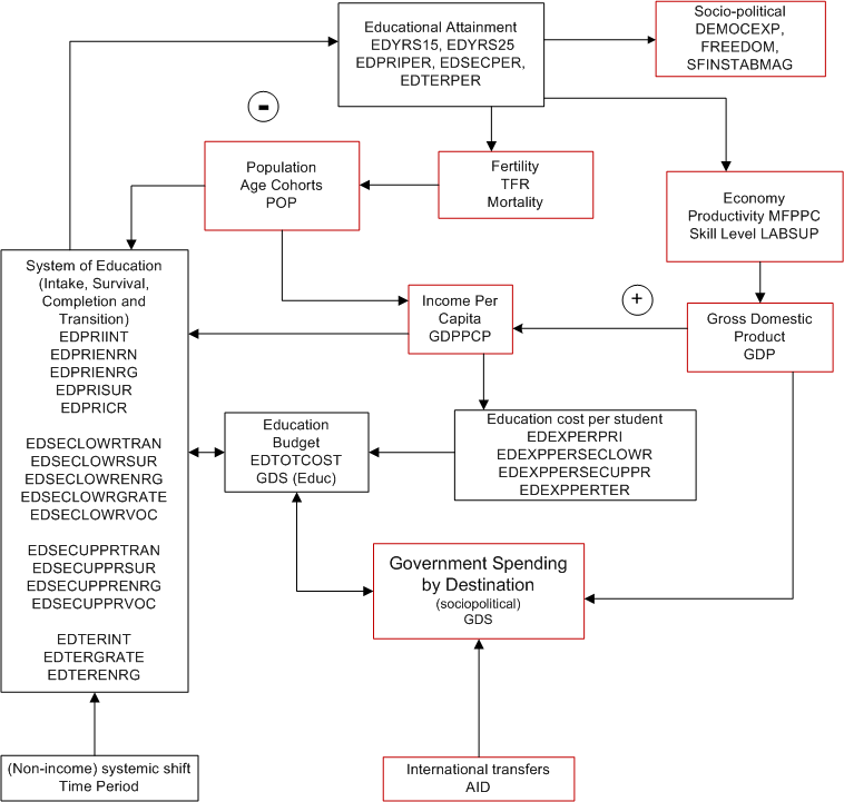
The education model has forward and backward linkages with other parts of the IFs model. During each year of simulation, the IFs cohort-specific demographic model provides the school age population to the education model.  In turn, the education model feeds its calculations of education attainment to the population model’s determination of women’s fertility.  Similarly, the broader economic and socio-political systems provide funding for education, and levels of educational attainment affect economic productivity and growth, and therefore also education spending. 

The figure below shows the major variables and components that directly determine education demand, supply, and flows in the IFs system.  The diagram attempts to emphasize on the inter-connectedness of the education model components and their relationship to the broader human development system.

Education Student Flow

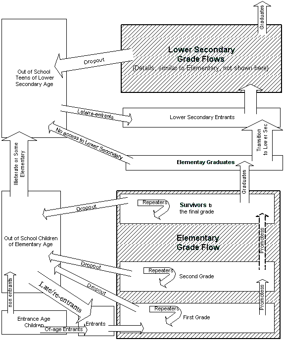
IFs education model simulates grade-by-grade student flow for each level of education that the model covers. Grade-by-grade student flow model combine the effects of grade-specific dropout, repetition and reentry into an average cohort-specific grade-to-grade flow rate, calculated from the survival rate for the cohort. Each year the number of new entrants is determined by the forecasts of the intake rate and the entrance age population. In successive years, these entrants are moved to the next higher grades, one grade each year, using the grade-to-grade flow rate. The simulated grade-wise enrollments are then used to determine the total enrollment at the particular level of education. Student flow at a particular level of education, e.g., primary, is culminated with rates of completion and transition by some to the next level, e.g., lower secondary.

The figure below shows details of the student flow for primary (or, elementary) level. This is illustrative of the student flow at other levels of education. We model both net and gross enrollment rates for primary. The model tracks the pool of potential students who are above the entrance age (as a result of never enrolling or of having dropped out), and brings back some of those students, marked as late/reentrant in the figure, (dependent on initial conditions with respect to gross versus net intake) for the dynamic calculation of total gross enrollments.

A generally similar grade-flow methodology models lower and upper secondary level student flows. We use country-specific entrance ages and durations at each level. As the historical data available does not allow estimating a rate of transition from upper secondary to tertiary, the tertiary education model calculates a tertiary intake rate from tertiary enrollment and graduation rate data using an algorithm which derives a tertiary intake with a lower bound slightly below the upper secondary graduation rate in the previous year.

Education Financial Flow

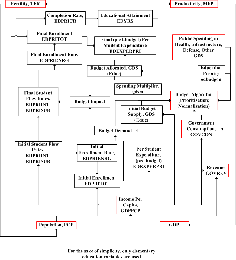
In addition to student flows, and interacting closely with them, the IFs education model also tracks financing of education. Because of the scarcity of private funding data, IFs specifically represents public funding only, and our formulations of public funding implicitly assume that the public/private funding mix will not change over time.

The accounting of educational finance is composed of two major components, per student cost and the total number of projected students, the latter of the two is discussed in the student flows section.  Spending per student at all levels of education is driven by average income. Given forecasts of spending per student by level of education and given initial enrollments forecasts by level, an estimate of the total education funding demanded is obtained by summing across education levels the products of spending per student and student numbers.

The funding needs are sent to the IFs sociopolitical model where educational spending is initially determined from the patterns in such spending regressed against the level of economic development of the countries. A priority parameter (edbudgon) is then used to prioritize spending needs over spending patterns. This parameter can be changed by model user within a range of values going from zero to one  with the zero value awarding maximum priority to fund demands. Finally, total government consumption spending (GOVCON) is distributed among education and other social spending sectors, namely infrastructure, health, public R&D, defense and an "other" category, using a normalization algorithm.

Government spending is then taken back to the education module and compared against fund needs. Budget impact, calculated as a ratio of the demanded and allocated funds, makes an impact on the initial projection of student flow rates (intake, survival, and transition). The positive (upward) side of the budget impact is non-linear with the maximum boost to growth occurring when a flow rate is at or near its mid-point or within the range of the inflection points of an assumed S-shaped path, to be precise. Impact of deficit is more or less linear except at impact ratios close to 1, whence the downward impact is dampened. Final student flow rates are used to calculate final enrollment numbers using population forecasts for relevant age cohorts. Finally, cost per students are adjusted to reflect final enrollments and fund availability.

Education Attainment

The algorithm for the tracking of education attainment is very straight-forward.  The model maintains the structure of the population not only by age and sex categories, but also by years and levels of completed education.  In each year of the model’s run, the youngest adults pick up the appropriate total years of education and specific levels of completed education.  The model advances each cohort in 1-year time steps after subtracting deaths. In addition to cohort attainment, the model also calculates overall attainment of adults (15+ and 25+) as average years of education  (EDYRSAG15, EDYRSAG25) and as share of people 15+ with a certain level of education completed (EDPRIPER, EDSECPER, EDTERPER).

One limitation of our model is that it does not represent differential mortality rates associated with different levels of education attainment (generally lower for the more educated).^[1] This leads, other things equal, to a modest underestimate of adult education attainment, growing with the length of the forecast horizon.  The averaging method that IFs uses to advance adults through the age/sex/education categories also slightly misrepresents the level of education attainment in each 5-year category.

1] The multi-state demographic method developed and utilized by IIASA does include education-specific mortality rates.

Education Equations

Overview

The IFs education model represent two types of educational stocks, stocks of pupils  and stocks of adults with a certain level of educational attainment . These stocks are initialized with historical data. The simulation model then recalculates the stock each year from its level the previous year and the net annual change resulting from inflows and outflows.

The core dynamics of the model is in these flow rates . These  flow rates are expressed as a percentage of age-appropriate population and thus have a theoretical range of zero to one hundred percent. Growing systems with a saturation point usually follow a sigmoid (S-shaped) trajectory with low growth rates at the two ends as the system begins to expand and as it approaches saturation. Maximum growth in such a system occurs at an inflection point, usually at the middle of the range or slightly above it, at which growth rate reverses direction. Some researchers (Clemens 2004; Wils and O’Connor 2003) have identified sigmoid trends in educational expansion by analyzing enrollment rates at elementary and secondary level. The IFs education model is not exactly a trend extrapolation; it is rather a forecast based on fundamental drivers, for example, income level. Educational rates in our model are driven by income level, a systemic shift algorithm and a budget impact  resulting from the availability of public fund. However, there are growth rate parameters for most of the flows that allow model user to simulate desired growth that follows a sigmoid-trajectory. Another area that makes use of a sigmoid growth rate algorithm is the boost in flow rates as a result of budget surplus.

Intake (or transition), survival, enrollment and completion are some of the rates that IFs model forecast. Rate forecasts cover elementary , lower secondary, upper secondary and tertiary levels of education with separate equations for boys and girls for each of the rate variables. All of these rates are required to calculate pupil stocks while completion rate and dropout rate (reciprocal of survival rate) are used to determine educational attainment of adults.

On the financial side of education, IFs forecast cost per student for each level. These per student costs are multiplied with enrollments to calculate fund demand. Budget allocation calculated in IFs socio-political module is  sent back to education model to calculate final enrollments and cost per student as a result of fund shortage or surplus.

The population module provides cohort population to the education model. The economic model provides  per capita income and the socio-political model provides budget allocation. Educational attainment of adults calculated by the education module affects fertility and mortality in the population and  health modules, affects productivity in the economic module and affects other socio-political outcomes like governance and democracy levels .

Equations: Student Flow

Econometric Models for Core Inflow and Outflow

Enrollments at various levels of education - EDPRIENRN, EPRIENRG, EDSECLOWENRG, EDSECUPPRENRG, EDTERENRG - are initialized with historical data for the beginning year of the model. Net change in enrollment at each time step is determined by inflows (intake or transition) and outflows (dropout or completion). Entrance to the school system (EDPRIINT, EDTERINT), transition from the lower level (EDSECLOWRTRAN, EDSECUPPRTRAN) - and outflows - completion (EDPRICR), dropout or it's reciprocal, survival (EDPRISUR) - are some of these rates that are forecast by the model.

The educational flow rates are best explained by per capita income that serves as a proxy for the families' opportunity cost of sending children to school. For each of these rates, separate regression equations for boys and girls are estimated from historical data for the most recent year. These regression equations, which are updated with most recent data as the model is rebased with new data every five years, are usually logarithmic in form. The following figure shows such a regression plot for net intake rate in elementary against per capita income in PPP dollars.

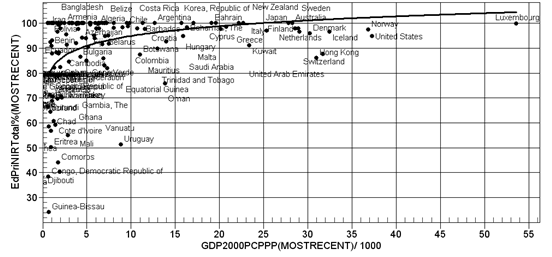
In each of the forecast years, values of the educational flow rates are first determined from these regression equations. Independent variables used in the regression equations are endogenous to the IFS model. For example, per capita income, GDPPCP, forecast by the IFs economic model drives many of the educational flow rates. The following equation shows the calculation of one such student flow rate (CalEdPriInt) from the log model of net primary intake rate shown in the earlier figure.

$CalEdPriInt_{g=1,r,t}=77.347+9.6372lnGDPPCP_{r,t}$

While all countries are expected to follow the regression curve in the long run, the residuals in the base year make it difficult to generate a smooth path with a continuous transition from historical data to regression estimation. We handle this by adjusting regression forecast for country differences using an algorithm that we call "shift factor" algorithm. In the first year of the model run we calculate a shift factor (EDPriIntNShift) as the difference (or ratio) between historical data on net primary intake rate (EDPRIINTN) and regression prediction for the first year for all countries. As the model runs in subsequent years, these shift factors (or initial ratios) converge to zero or one if it is a ratio (code routine ConvergeOverTime in the equation below) making the country forecast merge with the global function gradually. The period of convergence for the shift factor (PriIntN_Shift_Time) is determined through trial and error in each case.

$EdPriIntNShift_{g,r,t=1}=EDPRIINTN_{g,r,t=1}-CalEdPriInt_{g,r,t=1}$

$EDPRIINTN_{g,r,t}=CalEdPriInt_{g,r,t}+ConvergeOverTime(EdPriIntNShift_{g,r,t=1},0,PriIntNShiftTime)$

The base forecast on flow rates resulting from of this regression model with country shift is used to calculate the demand for funds. These base flow rates might change as a result of budget impact based on the availability or shortage of education budget explained in the budget flow section.

Systemic Shift

Access and participation in education increases with socio-economic developments that bring changes to people's perception about the value of education. This upward shifts are clearly visible in cross-sectional regression done over two adequately apart points in time. The next figure illustrates such shift by plotting net intake rate for boys at the elementary level against GDP per capita (PPP dollars) for two points in time, 1992 a

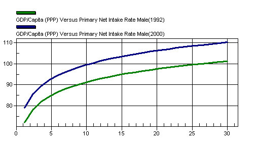
nd 2000.

IFs education model introduces an algorithm to represent this shift in the regression functions. This "systemic shift" algorithm starts with two regression functions about 10 to 15 years apart. An additive factor to the flow rate is estimated each year by calculating the flow rate (CalEdPriInt1 and CalEdPriInt2 in the equations below) progress required to shift from one function, e.g.,   to the other, s,  in a certain number of years (SS_Denom), as shown below. This systemic shift factor (CalEdPriIntFac) is then added to the flow rate (EDPRIINTN in this case) for a particular year (t) calculated from regression and country shift as described in the previous section.

$CalEdPriInt1_{g,r,t}=f_{1}(GDPPCP_{g,r,t})$

$CalEdPriInt2_{g,r,t}=f_{2}(GDPPCP_{g,r,t})$

$CalEdPriIntFac_{g,r,t}={\frac {t-1}{SSDenom}}*(CalEdPriInt2_{g,r,t}-CalEdPriInt1_{g,r,t})$

$EDPRIINTN_{g,r,t}=EDPRIINTN_{g,r,t}+CalEdPriIntFac_{g,r,t}$

As said earlier, Student flow rates are expressed as a percentage of underlying stocks like the number of school age children or number of pupils at a certain grade level. The flow-rate dynamics work in conjunction with population dynamics (modeled inside IFs population module) to forecast enrollment totals.

Grade Flow Algorithm

Once the core inflow (intake or transition) and outflow (survival or completion) are determined, enrollment is calculated from grade-flows. Our grade-by-grade student flow model therefore uses some simplifying assumptions in its calculations and forecasts. We combine the effects of grade-specific dropout, repetition and reentry into an average cohort-specific grade-to-grade dropout rate, calculated from the survival rate (EDPRISUR for primary) of the entering cohort over the entire duration of the level (EDPRILEN for primary). Each year the number of new entrants is determined by the forecasts of the intake rate (EDPRIINT) and the entrance age population. In successive years, these entrants are moved to the next higher grades, one grade each year, subtracting the grade-to-grade dropout rate (DropoutRate). The simulated grade-wise enrollments (GradeStudents with Gcount as a subscript for grade level) are then used to determine the total enrollment at the particular level of education (EDPRIENRG for Primary).

There are some obvious limitations of this simplified approach. While our model effectively includes repeaters, we represent them implicitly (by including them in our grade progression) rather than representing them explicitly as a separate category.  Moreover, by setting first grade enrollments to school entrants, we exclude repeating students from the first grade total.  On the other hand, the assumption of the same grade-to-grade flow rate across all grades might somewhat over-state enrollment in a typical low-education country, where first grade drop-out rates are typically higher than the drop-out rates in subsequent grades.  Since our objective is to forecast enrollment, attainment and associated costs by level rather than by grade, however, we do not lose much information by accounting for the approximate number of school places occupied by the cohorts as they proceed and focusing on accurate representation of total enrollment. 

$DropoutRate_{g,r,t}=1-({\frac {EDPRISUR_{g,r,t}}{100}})^{\frac {1}{\mathbf {EDPRILEN} _{r}-1}}$

$GradeStudents_{GCount=1,g,r,t}=EDPRIINT_{g,r,t}$

$GradeStudents_{Gcount,g,r,t}=GradeStudents_{Gcount-1,g,r,t}*(1-DropoutRate_{g,r,t})$

$EDPRIENRG_{g,r,t}=\sum _{Gcount=1}^{\mathbf {EDPRILEN} }GradeStudents_{Gcount,g,r,t}$

Gross and Net

Countries with a low rate of schooling, especially those that are catching up, usually have a large number of over-age students. Enrollment and entrance rates that count students of all ages are called gross rates in contrast to the net rate that only takes the of-age students in the numerator of the rate calculation expression. UNESCO report net and gross rates separately for entrance and participation in elementary. IFs education model forecasts both net and gross rate in primary education. An overage pool (PoolPrimary) is estimated at the model base year using net and gross intake rate data. Of-age non-entrants continue to add to the pool (PoolInflow). The pool is exhausted using a rate (PcntBack) determined by the gross and net intake rate differential at the base year. The over-age entrants (cOverAgeIntk_Pri) gleaned from the pool are added to the net intake rate (EDPRIINTN) to calculate the gross intake rate (EDPRIINT).

$PoolPrimary_{r,g,t=1}=f(EDPRIINTN_{g,r,t=1},EDPRIINT_{g,r,t=1})$

$PcntBack_{r,g}=f(PoolPrimary_{r,g,t=1},EDPRIINTN_{g,r,t=1},EDPRIINT_{g,r,t=1})$

$PoolInflow=f(EDPRIINTN_{g,r,t})$

$cOverAgeIntkPri=f(EDPRIINTN_{g,r,t},PoolPrimary_{g,r,t},PcntBack_{r,g})$

$PoolPrimary_{r,g,t}=PoolPrimary_{r,g,t-1}+PoolInflow-cOverAgeIntkPri$

$EDPRIINT_{g,r,t}=EDPRIINTN_{g,r,t}+cOverAgeIntkPri$

Vocational Education

IFs education model forecasts vocational education at lower and upper secondary levels. The variables of interest are vocational shares of total enrollment in lower secondary (EDSECLOWRVOC) and the same in upper secondary (EDSECUPPRVOC). Country specific vocational participation data collected from UNESCO Institute for Statistics do not show any common trend in provision or attainment of vocational education across the world. International Futures model initialize vocational shares with UNESCO data, assumes the shares to be zero when no data is available and projects the shares to be constant over the entire forecasting horizon. 

IFs also provides two scenario intervention parameters for lower (edseclowrvocadd) and upper secondary (edsecupprvocadd) vocational shares. These parameters are additive with a model base case value of zero. They can be set to negative or positive values to raise or lower the percentage share of vocational in total enrollment. Changed vocational shares are bound to an upper limit of seventy percent. This upper bound is deduced from the upper secondary vocational share in Germany, which at about 67% is the largest among all vocational shares for which we have data. Changes to the vocational share through the additive parameters will also result in changes in the total enrollment, e.g., EDSECLOWRTOT for lower secondary, which is calculated using general (non-vocational) enrollment (EdSecTot_Gen) and vocational share, as shown in the equations below (for lower secondary).

$EDSECLOWRVOCI_{g,r}=EDSECLOWRVOC_{g,r,t=1}$

$EDSECLOWRVOC_{g,r,t}=EDSECLOWRVOCI_{g,r}+edseclowrvocadd_{g,r,t}$

$EDSECLOWRTOT_{g,r,t}={\frac {EdSecTotGen_{g,r,t}}{1-{\frac {EDSECLOWRVOC_{g,r,t}}{100}}}}$

Forecasts of EdSecTot_Gen_g,r,t  is obtained in the full lower secondary model using transition rates from primary to lower secondary and survival rates of lower secondary.

Science and Engineering Graduates in Tertiary

Strength of STEM (Science, Technology, Engineering and Mathematics) programs is an important indicator of a country’s technological innovation capacities. IFs education model forecasts the share of science and engineering degrees (EDTERGRSCIEN) among all tertiary graduates in a country. Data for this variable is available through UNESCO Institute for Statistics. The forecast is based on a regression of science and engineering share on average per person income in constant international dollar (GDPPCP). There is an additive parameter (edterscienshradd), with a base case value of zero, that can be used to add to (or subtract from) the percentage share of science and engineering among tertiary graduates. This parameter does not have any effect on the total number of tertiary graduates (EDTERGRADS).

$EDTERGRSCIEN_{r,t}=f(GDPPCP_{r,t})+edterscienshradd_{r,t}$

Equations: Budget Flow

Resources required to maintain the projected student flows are determined by multiplying enrollment rates with per student cost forecasts. Availability of resources, as determined in the IFs socio-political model, affect flow rates and the final enrollment rate.

Public expenditure per student (EDEXPERPRI) as a percentage of per capita income is first estimated (CalExpPerStud) using a regression equation. Country situations are added as a shift factor (EdExPerPriShift) that wears off over a period of time (edexppconv) in the same manner as those for student flow rates. The following group of equations show the calculation of per student expenditure in primary (EDEXPERPRI).

$CalExpPerStud_{r,t}=f(GDPPCP_{r,t})$

$EdExpPerPriShift_{r,t=1}=EDEXPERPRI_{r,t=1}-CalExpPerStud_{r,t=1}$

$EDEXPERPRI_{r,t}=CalExpPerStud_{r,t=1}+ConvergeOverTime(EdExpPerPriShift_{r,t=1},0,\mathbf {edexppconv} )$

Total fund demand (EDBUDDEM, see calculation below) is passed to the IFs socio-political model where a detail government budget model distributes total government consumption among various public expenditure sectors. For education allocation, an initial estimate (gkcomp) is first made from a regression function of educational spending as a percentage of GDP over GDP per capita at PPP dollars (GDPPCP) as a country gets richer. 

$gkcomp_{r,Educ,t}=f(GDPPCP_{r,t})$

Like several other functions discussed in this sub-module, country situation is reflected by estimating country ratio (gkri) between the predicted and historical value in the base year. This ratio converges to a value of one very slowly essentially maintaining the historic ratio. Public spending on education in billion dollars (GDS) is then calculated using the regression result, GDP and the multiplicative shift.

$gkri_{r,Educ}=GDS_{r,Educ,t=1}/GDP_{r,t=1}/gkcomp_{r,Educ,t=1}$

$gkshift_{r,t,Educ}=ConvergeOverTime(gkri_{r,Educ},200,1)$

$GDS_{r,Educ,t}=gkcomp_{r,Educ,t}*gkshift_{r,t,Educ}*GDP_{r,t}/100$

Sociopolitical model also forecast public spending in other areas of social spending, i.e., military, health, R&D. Another public spending sector, infrastructure is calculated bottom-up, i.e., as an aggregation of demand for construction and maintenance of various types of infrastructure.

Once all the spending shares are projected, a normalization algorithm is used to distribute the total available government consumption budget (GOVCON) among all sectors.

$GTOT=\sum _{s=1}^{NGovExp}GDS_{r,s}$

$GDS_{r,s}={\frac {GDS_{r,s}}{GTOT}}*GOVCON_{r,s}$

Before normalization, a priority parameter allows setting aside all or part of fund demands for the ground up spending sectors, i.e., infrastructure and education. For education sector, the prioritization parameter (edbudgon) is used to set aside a certain portion of the projected education investment as shown in the equations below.

$GDSSetAside=GDS_{r,Educ}*(1-\mathbf {edbudgon} )$

$GDS_{r,Educ}=GDS_{r,Educ}-GDSSetAside$

Education allocation, GDS (Educ) calculated thus is taken back to the education model. A second normalization and prioritization is done within the education model to distribute total education allocation among different levels of education. This across level normalization uses the percentage share of each educational level in the total demand for education funding. First, total expenditure demand for all levels of education combined is determined by multiplying the total enrollments with per student costs. The following equation shows the calculation for Primary. 

$BudDemPri_{r,t}=UDEDExpPerPri_{r,t}*GDPPCP_{r,t}*\sum _{g=1}^{2}UDEnrollCT_{r,t}/100$

Fund demands for all levels are added up to get the total fund demand under no budget constraint. The prefixes UD here stands for budget unconstrained demand.

$EDBudDem_{r,t}=BudDemPri_{r,t}+BudDemSecLowr_{r,t}+BudDemSecUppr_{r,t}+BudDemTer_{r,t}$

Any surplus or deficit in educational allocation, calculated as the difference between education sector allocation in the government budget model and the total fund requirement for all levels of education combined, first undergoes an adjustment algorithm that boosts (in case of surplus) or reduces (in case of deficit) per student cost for those countries which are below or above the level they are supposed to be. Post this adjustment, allocation is distributed across all levels using a normalization process based on demand.  

A budget impact ratio  is then calculated as the ratio of the fund demanded (CalcTotCost) and fund obtained (CalcTotSpend). This budget impact ratio (CalcBudgetImpact)  increases or decreases the pre-budget (or demand side as we call it) projection of student flow rates (intake, survival, and transition). The positive (upward) side of the budget impact is non-linear with the maximum boost to growth occurring when a flow rate is at or near its mid-point or within the range of the inflection points of an assumed S-shaped path, to be precise. Impact of deficit is more or less linear except at impact ratios close to 1, whence the downward impact is dampened. Final student flow rates are used to calculate final enrollment numbers using population forecasts for relevant age cohorts. Finally, cost per students are adjusted to reflect final enrollments and fund availability.

Budget impacts uses a non-linear algorithm intended to generate an S-shaped growth rate. Final enrollment is then calculated from this final flow rates and any of the remaining budget is used to increase per student expenditure.

$CalcTotCost=(EDEXPERPRI_{r}/100)*GDPPC_{r}*convtoexchange*\sum _{g=1}^{2}EDPRITOT_{r,g}$

$CalcTotSpend=GDS_{r,Educ}*GDSED_{r,Pri}/SpendCostRI$

In the equations above, convtoexchange is a factor that converts monetary units from PPP to exchange rate dollars, SpendCostRI is a ratio calculated at the first year of the model to reconcile historical data on aggregate and bottom-up spending.

$CalcBudgetImpact=CalcTotSpend/CalcTotCost$

$EDPRIINTN_{g,r,t}=f(EDPRIINTN_{g,r,t},CalcBudgetImpact)$

$EDPRISUR_{g,r,t}=f(EDPRISUR_{g,r,t},CalcBudgetImpact)$

Equations: Attainment

There are two types of variables that keep track of educational attainment: average years of education of adults (EDYRSAG15, EDYRSAG15TO24 and EDYRSAG25) and percentage of adults with a certain level of education (EDPRIPER, EDSECPER, EDTERPER). Both groups forecast attainment by gender.

The basis of calculation for both groups of variables is educational attainment by age cohort and gender as contained in intermediate model variables, EDPriPopPer _r.g,c,t ,  EDSecPopPer_r.g,c,t, EdTerPopPer_r.g,c,t (where, r stands for country or region, g for gender, c for cohort and t for time).

We initialize attainments of the entire adult population (EDPRIPER, EDSECPER, EDTERPER) using historical data estimated by Barro and Lee (2000) and use a spread algorithm. The spread algorithm starts with the most recent data on school completion rate (EDPRICR for primary) which is considered as the average attainment of the graduating cohort. The algorithm then uses the differential between that completion rate and the attainment rate of the adults (EDPRIPER) to back calculates a delta reduction for each of the older cohorts (EdPriPopPer) such that averaging attainments over cohorts one can obtain average attainment for all adults (EDPRIPER).

$EDPriPopPer_{c,g,r,t=1}=f(EDPRIPER_{r,g,t=1},EDPRICR_{r,g,t=1})$

where, subscript c stand for five year age cohorts going from 1 to 21. Cohort 4, represents the 15 to 19 years and NC, total number of age cohorts.

For subsequent forecast years, cohort educational attainment for each level of education is calculated by adding graduates from that level of education to the appropriate age cohort, advancing graduates from the younger cohort, and passing graduates to the older cohort. 

$EDPriPopPer_{c=pc,g,r,t}=0.8*EDPriPopPer_{c=pc,g,r,t-1}+0.2*EDPRICR_{g,r,t}$

where, pc stands for the five year age cohort where the primary graduates belong. For all other cohorts:

$EdPriPopPer_{c,g,r,t}=0.8*EdPriPopPer_{c,g,r,t-1}+0.2*EdPriPopPer_{c-1,g,r,t-1}$

Cohort attainments for secondary and tertiary education (EDSECPOPPER, EDTERPOPPER) are initialized and forecast in a similar fashion. An average years of education reflecting completion of levels is then calculated by from the cohort attainment, population and cohort length as shown in the next equation where   AGEDST_c,g,r,t contains the population of five year age cohorts and EDPRILEN _r,t   is the duration of primary cycle in years.

$AvgYearsPriEdPop_{g,r,t}={\frac {\sum _{c=pc}^{NCohorts}{\frac {EDPriPopPer_{c,g,r,t}}{100}}*EDPRILEN_{r}*AGEDST_{c,g,r,t}}{\sum _{c=pc}^{NCohorts}AGEDST_{c,g,r,t}}}$

For those who dropout before completing a certain level we need to calculate the partial attainment and add that to the average years of education. The average of the partial years of education at a particular year is calculated from dropouts by level and grade as shown below. Calculation of the average of partial years resulting from dropouts in primary education is illustrated in the equations below. Partial years from current year dropouts at other levels of education are calculated in the same manner and all the partial years are averaged to an overall average. This new partial attainment is then added to the partial attainment of five year cohorts which are initialized and advanced in a similar manner as that used for cohort averages on completed attainment.

$DropoutRate_{g,r,t}=f(EDPRISUR_{g,r,t},\mathbf {EDPRILEN} _{r})$

$GrStudents_{GCount,g,r,t}=f(EDPRIINT_{g,r,t},DropoutRate_{g,r,t},\mathbf {EDPRILEN} _{r})$

$PartialPriPersYearsNew_{g,r,t}={\frac {(\sum _{GCount=2}^{EDPRILEN_{r}}GrStudents_{GCount,g,r,t}*DropoutRate_{g,r,t}*(GCount-1))*\mathbf {\sum _{c=EDPRISTART}^{EDPRILEN}} FAGEDST_{g,r,t}}{\mathbf {\sum _{c=EDPRISTART}^{EDPRILEN}} FAGEDST_{g,r,t}}}$

Here,  EDPRISUR is the survival rate in primary education, EDPRISTART is the official entrance age for primary schooling, Gr_Students is the enrollment at a certain grade, GCount is the grade counter and FAGEDST is the population of the single year age cohort corresponding to the grade level. 

Overall attainment, i.e., average years of education are calculated by averaging the attainments and partial attainments of five year age cohorts as shown in the equation below. The suffixes on the variables EDYRSAG15, EDYRSAG15TO24 and EDYRSAG25 indicate the age thresholds at which or the age bracket over which attainment is averaged.

$EDYRSAG15_{g,r,t}=AvgYearsPriEdPop_{g,r,t}+AvgYearsSecEdPop_{g,r,t}+AvgYearsTerEdPop_{g,r,t}+PartialYearsEdPop_{g,r,t}$

Attainments by level, i.e., EDPRIPER, EDSECPER and EDTERPER are also obtained by summing across the corresponding five year cohorts, i.e., EdPriPopPer etc.

$EDPRIPER_{g,r,t}={\frac {\sum _{c=4}^{NCohorts}EdPriPopPer_{c,g,r,t}*AGEDST_{c,g,r,t}}{\sum _{c=4}^{NCohorts}AGEDST_{c,g,r,t}}}$

Cohort attainments by level of education are also used in to build a specialized educational attainment display, commonly referred to as education pyramid in congruence with demographic pyramids used to display population by age cohorts stacked one on top of the other with the men and women cohorts put opposite to each other around a vertical axis. Education pyramid superimposes educational attainment on top of the demographic pyramid. 

Knowledge Systems

Overview

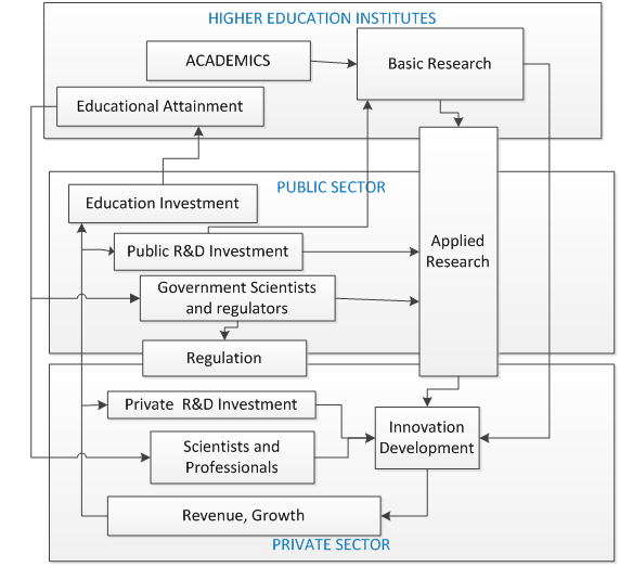
Knowledge and innovation are important drivers of  economic growth and human well-being. These activities also  help societies address major social and environmental challenges. Education and research and a linear relationship between these and product development are no longer considered a good model of knowledge and innovation systems. However, the linear model was the first successful attempt (Bush, V, 1945) in conceptualizing the science, technology and innovation (STI) activities. One of the major contributions of these first models was the distinction between basic and applied researches and the identification of stakeholders and funding for each type as shown in the next figure.

The failure of the linear model to capture the intricacies and interactions involved in the innovation process and the broader role of the public and private institutions and individuals in facilitating creation and diffusion of knowledge prompted some experts to resort to rich qualitative description of so called “national systems of innovation” starting from late 1980s, early 1990s. Increased educational attainment, fast expansion of information and communication technologies, more sophisticated production technologies and an expansion in the exchange of goods, ideas and people over the last few decades tell of something broader than just innovation constrained within national boundaries. Recent literature (citation) use concepts like knowledge economy or knowledge society to describe the systemic nature and impact of knowledge-intensive activities.

This new literature takes an evolutionary perspective and talks about a gradual unfolding of knowledge and innovation system (citation: Nelson, Freeman etc) within a country marked by a certain types of actors, institutions and organizations and the linkages across and within such components. Studies in this area range from more focused concepts of knowledge economy (citation: WB; OECD) to a broader knowledge society (citation: UNESCO; Bell), from a more qualitative innovation systems approach (citation: Nelson; Freeman) to a measurement focused innovation capacity approach (citation: GII Dutta, Archibucchi..). The complementarity of the components of such a system demands that the components be studied together. Accordingly, experts have come up with composite indices for assessing the knowledge and innovation capacities of countries around the world. Such indices give a good idea of the overall status of the innovation capacities of the country and the stage of knowledge society it is in. The components of the composite indices are categorized across four to five major dimensions (or, pillars, as some studies call these), for example, education and skills, information infrastructure, institutional regime, innovation activities (WB Knowledge Index etc).

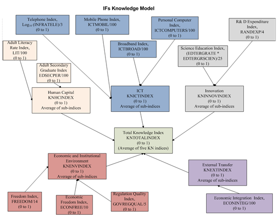
International Futures (IFs) Knowledge module builds on other knowledge systems measurement approaches (cite WB KEI here) by designing a composite knowledge index (KNTOTALINDEX) comprised of five sub-indices containing a total of (x) components. The indices and the sub-indices are then forecast over the entire IFs’ horizon by combining the components which are themselves forecast through different modules of the integrated IFs model. To our knowledge, IFs is the only model capable of making such an organic forecast of the knowledge capacity of a country.

IFs Knowledge Indices

The capacity of a society to tap from and add to the pool of existing knowledge, local and global, depends on

• skills and qualifications of people to assimilate existing and new knowledge,
• an innovation system to facilitate development or adoption of of new knowledge, processes and products
• a technological infrastructure to share, disseminate and regenerate knowledge and information within and across societies
• political and institutional environment conducive to the generation, diffusion and utilization of knowledge
• regulations that offer appropriate incentives towards and remove barriers from international transfer of knowledge

The above list of the driving dimensions of a knowledge system is exhaustive, to the best of our knowledge. The list has five dimensions contrasted to the four pillars identified by the WB KAM. However, World Bank includes tariff & non-tariff barriers, an indicator of international transfer, in their fourth pillar on economic and institutional environment. 

IFs now has five indices representing the five dimensions described above. The details of each of these indices, and a sixth one averaged from these five, will be described later. Suffice here to say that, the indices are calculated each of the forecast years by averaging the forecasted value of relevant IFs variables, normalized over a continuous interval going from 0 to 1. That is, IFs integrated simulation, first, forecasts a specific variable, e.g., adult literacy rate, it then converts the forecast to a normalized value lying between zero to one and then averages one or more of these normalized values to obtain an index along each of the dimensions of knowledge assessment. The table below compares IFs knowledge indices with those from World Bank. 

No.	Dimension/Pillar	World Bank Variables	IFs Index	IFs Variables
1	Human Capital	Adult literacy rate; Secondary enrollment rate; Tertiary enrollment rate	KNHCINDEX	Adult literacy rate; Adult secondary graduation rate
2	Innovation	R&D researchers, Patent count; Journal articles (all per million people)	KNINNOVINDEX	Total R&D expenditure (% of GDP); Tertiary graduation rate in science and engineering
3	ICT	Telephones (land + mobile) per 1000 persons; Computers per 1000 persons; Internet users per 10000 persons	KNICTINDEX	Telephone (fixed); Mobile phone; Personal Computers; Broadband
4	Economic and Institutional Regime	Tariff and non-tariff barriers; Regulatory quality; Rule of law	KNENVINDEX	Freedom; Economic freedom; Government regulation quality
5	International Transfer of Knowledge		KNEXTINDEX	Economic integration index
6	Composite Index	Knowledge Index, KI (from the first three) and Knowledge Economy Index, KEI (from all 4)	KNTOTALINDEX	From all of the above

Knowledge Systems Equations: Total Knowledge Index

The composite index (KNTOTALINDEX) consists of five sub-indices, of which the first four contains national actors and institutions only. The fifth one, international transfer index (KNEXTINDEX), attempts to capture the impact of global knowledge flows through a measure of the country’s openness to the international system. The first four sub-indices - human capital (KNHCINDEX), information infrastructure (KNICTINDEX), innovation systems (KNINNOVINDEX) and governance and business environment (KNENVINDEX) – will be described below. The external index (KNEXTINDEX) is given a somewhat lower weight in the total index than the other four sub-indices which are equally weighted to a total of 90% of the total index. KNEXTINDEX itself is constructed from two equally weighted components of international trade and foreign direct investment.

$KNTOTALINDEX_{r,t}=0.9*{\frac {(KNHCINDEX_{r,t}+KNICTINDEX_{r,t}+KNINNOVINDEX_{r,t}+KNENVINDEX_{r,t})}{4}}+0.1*(KNEXTINDEX_{r,t})$

Knowledge Systems Equations: Knowledge Sub-Indices

In this section we describe the calculation method for various IFs knowledge indices. 

Human capital Index: KNHCINDEX

The purpose of this index is to capture the cross-country differences in the productive capacity of an average worker. We use two educational stock variables for the purpose. Differences in the rate of literacy, the sheer ability to read or write, make a big difference in productivity in more traditional type and/or informal activities. As the countries move gradually a more traditional agricultural economy to comparatively higher value added activities, e.g., assembling machineries or running a call center, secondary education become more important. The index is built through a combination of two sub-indices: literacy index, LitIndex and secondary attainment index, AdultSecPerIndex, weighted equally.

This index could be improved by adding a measure of the quality of education and an indicator of the skill-base of the worker. Unfortunately, IFs forecasts on those two areas are limited or non-existent at this point. [Note: The sub-indices – LitIndex and AdultSecPerIndex – used for this and other knowledge indices are calculated only in the model code. They are not available for display.]

$KNHCINDEX_{r,t}=(LitIndex_{r,t}+AdultSecPerIndex_{r,t})/2$

Literacy index, with a theoretical range of values from 0 to 1, is calculated by dividing literacy rate, LIT, which can range from 0 to 100, by 100. 

$LitIndex_{r,t}=LIT_{r,t}/100$

For the sub-index on secondary attainment (percentage of adults with completed secondary education), we use a similar normalization algorithm like the literacy sub-index. 

$AdultSecPerIndex_{r,t}=EDSECPER_{r,total,t}/100$

LIT and EDSECPER are forecast in the IFs population and education modules.

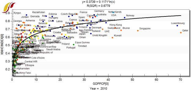
Because it excludes any measure of higher education which is included in the innovation sub-index (KNINNOVINDEX) described below, KNHCINDEX turns out to be very useful in showing the differences across developing countries. Even for richer countries, most of which achieved near universal secondary enrollment and universal literacy, the index shows significant variance coming from the secondary attainment differences among the elderly.

Innovation Index: KNINNOVINDEX

This IFs knowledge sub-index measures the innovation capacity of a nation through its R&D inputs – resources and personnel. It comprises of a total R&D expenditure index and a tertiary science and engineering graduation index as shown in the equations below.

$KNINNOVINDEX_{r,t}=(RandDExpIndex_{r,t}+EdTerGrateIndex_{r,t})/2$

For R&D expenditure, the highest spenders like Israel and Finland, spend close to or little over 4% of GDP and we use that number as a maximum to normalize all other countries in a zero to one range.

$RandDExpIndex_{r,t}=RANDDEXP_{r,t}/4$

For science and engineering graduation rate, 25% is used as a maximum. The equations below show the calculation which uses tertiary graduation percentage, EDTERGRATE _Total and the share of total graduates that obtain a science or engineering degree, EDTERGRSCIEN, both of which are forecast in the IFs education model.

$EdTerGrateIndex_{r,t}=EDTERGRATE_{r,total,t}*{\frac {EEDTERGRSCIEN_{r,t}}{100}}/25$

ICT Index: KNICTINDEX

Information and communication technologies (ICT) have a very significant role in facilitating the creation and diffusion of knowledge. IFs knowledge sub-index on ICT is built from the diffusion rates of core ICT technologies mobile, landline, broadband and a personal computer access rate sub-index. The telephone lines (fixed lines) sub-index, unlike the other three, use the logarithm of telephone line access rates as the differences in impacts of plain old telephone system decreases at higher access rates. In fact, the gradual shift from a wired to a wireless line as a personal communication device, demands that we reconsider the inclusion of this component in the ICT index.

$KNICTINDEX_{r,t}=(ICTTelephoneIndex_{r,t}+ICTMobileIndex_{r,t}+ICTBroadIndex_{r,t}+ICTComputersIndex_{r,t})/4$

$ICTTelephoneIndex_{r,t}=log(INFRATELE_{r,t})/3$

$ICTMobileIndex_{r,t}=ICTMOBIL_{r,t}/100$

$ICTBroadIndex_{r,t}=ICTBROAD_{r,t}/100$

$ICTComputersIndex_{r,t}=ICTCOMPUTERS_{r,t}/100$

Governance and Regulatory Environment: KNENVINDEX

The existence of economic and regulatory institutions and an effective governance of such institutions are important for generation, diffusion and utilization of knowledge. IFs knowledge sub-index representing these, KNENVINDEX, is calculated from three sub-indices which are themselves indices forecast by other IFs modules. These indices, one for economic freedom, a second one for overall freedom in the society and a third one on governance regulatory quality are each normalized to a 0 to 1 scale and averaged to get KNENVINDEX.

For the variables economic freedom, political freedom and governance regulation quality and average them to KNENVINDEX.

$KNENVINDEX_{r,t}=(EconFreeIndex_{r,t}+FreeDomIndex_{r,t}+GovRegQualIndex_{r,t})/3$

$EconFreeIndex_{r,t}=ECONFREE_{r,t}/10$

$FreeDomIndex_{r,t}=FREEDOM_{r,t}/14$

$GovRegQualIndex_{r,t}=GOVREGQUAL_{r,t}/5$

International Transfer Index: KNEXTINDEX

KNEXTINDEX attempts to represent cross-national knowledge flows, a major phenomenon in today’s globalized world. The more open a country is the more likely it is for her to learn from the global advancements in science, technology and other forms of knowledge. The sub-index that IFs calculates uses two indicators, trade and foreign direct investment (FDI). FDI indicator is given twice the weight given to trade volume.

$KNEXTINDEX_{r,t}=(TradeIndex_{r,t}+2*InvIndex_{r,t})/2$

$TradeIndex_{r,t}=log{\frac {XRPA_{r,t}+MRPA_{r,t}}{GDPPOT_{r,t}}}/log1000$

$InvIndex_{r,t}=log{\frac {XFDISTOCK_{r,t}+XFDISTOUT_{r,t}}{GDPPOT_{r,t}}}/log500$

Barro-Lee Education Data </div>