Water model documentation

The water model of the International Futures (IFs) system forecasts water demand by sector (municipal, industrial, and agricultural) and supply by source (surface water, groundwater, non-renewable groundwater, desalinated water, and treated wastewater) for 186 countries to the year 2100. Water supply and demand are equilibrated using a shadow price index, which is determined using a proportional-integral-derivate (PID) controller. There are no “forward linkages” from the water model to the rest of the IFs system; however, user-controlled parameters allow water scarcity to impact agricultural yields.

Introduction

Dominant Relations

We model water demand as the sum of the water demand of three sectors—municipal, industrial, and agriculture. The data we use from AQUASTAT differentiates between these three sectors and many other water models that use these same sectors. AQUASTAT refers to these data series as “water withdrawal.” For our purposes, we consider water withdrawal to be equivalent to water demand.

Water supply is defined as the sum of five components: surface water withdrawal, renewable groundwater withdrawal, non-renewable (fossil) water withdrawal, desalinated water, and direct use of treated wastewater.

The size of a country’s urban population and water use per capita for the urban population drive municipal water demand. Water use per capita for the urban population is driven by GDP per capita (at purchasing power parity), the portion of the population with access to piped water, and the portion of the population that lives in urban areas. Non-renewable electricity generation capacity and the overall size of a country’s manufacturing sector drive industrial water demand. The area of land under irrigation drives agricultural water demand. The shadow price index impacts all three water demand sectors.

Surface and (renewable) groundwater withdrawals are driven by the shadow price index and constrained by their country-specific exploitable limits. Estimated stocks constrain fossil water withdrawals. The price index and an initial growth rate (which can be specified by user) drive desalinated water. Direct use of treated wastewater is driven by the price index and the volume of wastewater which is treated.

Total water demand and total water supply are used to adjust the price index. The water price  index then impacts each sector of demand and most sources of supply the following year. This algorithmic logic keeps water demand and water supply in approximate equilibrium over time, even though it does not require exact equality in any time step.

Structure and Agent System

System/Subsystem	Environment (e.g. CO2, water)
Organizing Structure	Systemic Accounting
Stocks	Exploitable renewable water resources (surface and ground)   Total renewable water resources (surface and ground)   Non-renewable (fossil) water   Water price index
Flows	Water demand (municipal, industrial, agriculture)   Wastewater (produced, treated, treated and reused)   Desalinated water   Non-renewable (fossil) water withdrawal
Key Aggregate  Relationships  (illustrative, not comprehensive)	Water withdrawals as a portion of exploitable limit   Water price index
Key Agent-Class Behavior  Relationships (illustrative, not comprehensive)	Governments and environmental policies regarding exploitable limits   Water demand and supply responses to scarcity (elasticities on sectors)

Water Flow Charts

Water Overview

Water supply and demand as equilibrated using a water price index.

 

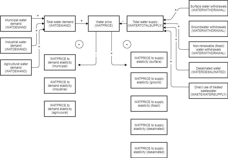
Water Demand Overview 

Three components of water demand: municipal, industrial, and agriculture.

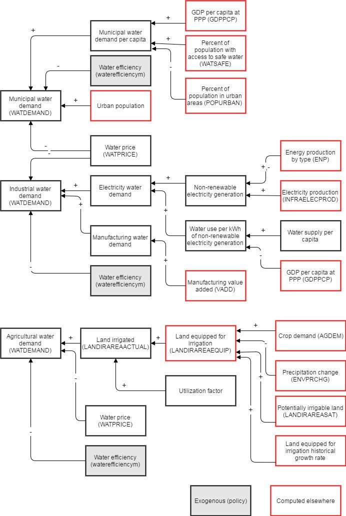
Water Supply Overview

Five components of water supply and their driving variables.

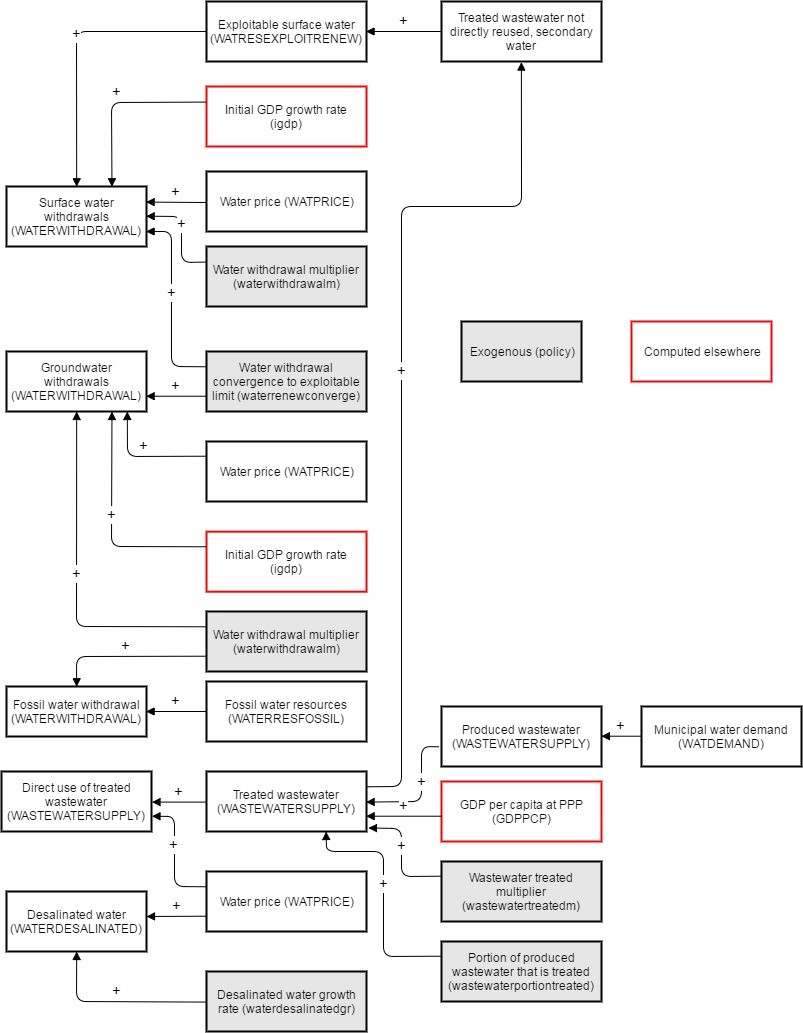
Forward linkages

Conceptual framework for water constraints on the agriculture model

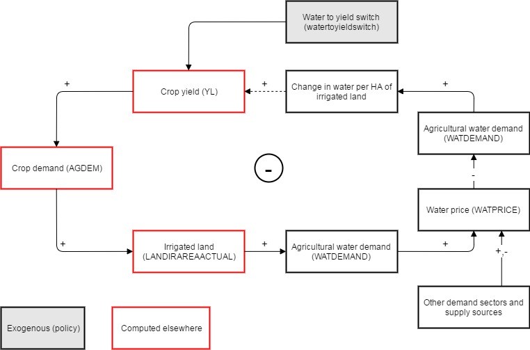
Water Equations

Water Demand

Water demand is disaggregated into three sectors: agricultural, municipal, and industrial. Each of these three sectors have their own driving variables, mainly calculated in other sub-modules of the IFs model. Each of the equations for the three sectors of demand follow roughly the same structure – the first term in each of the equations is a level of water withdrawal intensity (water use per HA of irrigated land, municipal water use per capita, and water use per kWh of non-renewable electricity generation). This term is then multiplied by the overall size of the denominator in each of these intensity calculations (area of irrigated land, urban population, and non-renewable electricity generation).

Each sector of water demand is also impacted by changes in the water price index using a -0.1 elasticity (see section on water price index for details on those calculations).

$WATDEMAND_{r,municipal,t+1}=WATDEMAND_{r,municipal,t}*(1+(IncreaseInPrice_{r}*-0.1))$

$WATDEMAND_{r,industrial,t+1}=WATDEMAND_{r,industrial,t}*(1+(IncreaseInPrice_{r}*-0.1))$

$WATDEMAND_{r,agriculture,t+1}=WATDEMAND_{r,agriculture,t}*(1+(IncreaseInPrice_{r}*-0.1))$

Agricultural water demand

Water use for irrigation can be estimated by the following equation:

$WI=AEI*UIA*WRCI*{\frac {1}{IE}}$

Where WI is the water demand for irrigation (m³), AEI is the area equipped for irrigation (HA), UIA is the utilization intensity of irrigated land, i.e., the ratio of irrigated land actually irrigated over extent of land equipped for irrigation, and WRCI is the total crop water requirement per unit of irrigated area depending on climate, crop type and multi-cropping conditions, and can be affected by specific crop management practices. IE is the efficiency of irrigation that accounts for the losses during water transport and irrigation application, (Wada et al., 2015).

Forecasting irrigation water demand thus requires forecasting these four components.

Area equipped for irrigation (AEI)

The area of land equipped for irrigation is driven by sub-national factors (mostly biophysical), and national factors (socio-political and governance related) (Neumann et al., 2011; Wada et al., 2016). Wada et al. identify nine potential drivers for the area of land equipped for irrigation: availability of land and water; reliability of water supply and access to water; irrigation impact (achievable yield increase and/or stabilization of yields and reduced variability); agricultural demand; availability of land with rain-fed potential; existing current yield gaps in rain-fed and/or irrigated land; cost; profitability, economic means available and support policies to invest in irrigation; state food security and self-reliance policies (Wada et al., 2015).

Neumann et al., (2011) modelled global irrigation patterns using a multilevel approach, using driving variables at the grid level as well as the national level. At the national level, they identified the following variables as significant: corruption, government effectiveness, GDP, political stability, autocracy, democracy. Many of these variables are correlated, so the authors of that paper used the variables, “government_performance” and “government_type” in their final analysis. At the grid level, Neumann et al. found the following variables to be significant: slope discharge; humidity; evaporation; evapotranspiration; population density; and access to markets.

Because the IFs system uses countries (or provinces in some cases) as the unit of analysis, we are unable to incorporate indicators at the grid level. In an effort to account for these grid-level indicators, we have incorporated data on the area of potentially irrigable land into our model. “Irrigation potential” is defined by AQUASTAT as

Area of land which is potentially irrigable. Country/regional studies assess this value according to different methods. For example, some consider only land resources, others consider land resources plus water availability, others include economical aspects in their assessments (such as distance and/or difference in elevation between the suitable land and the available water) or environmental aspects, etc. If available, this information is given in the individual country profiles. The figure includes the area already under agricultural water management.

Using this variable (% of potential) as the dependent variable, implicitly includes some of the constraining factors identified above in the analysis. For example, while we do not include land availability and the slope of the land as explicit driving variables, those factors limit the area of potentially irrigable land.

For independent variables, we used crop demand and precipitation (see metadata below):

SeriesLandIrAreaEquip

• Definition: Area equipped for irrigation: total (1000 HA)
• Source: AQUASTAT
• Units: 1000 ha

SeriesLandIrPotential

• Definition: Irrigation potential (1000 ha)
• Source: AQUASTAT
• Units: 1000 ha

SeriesEnvPrecipitation

• Definition: Average annual precipitation from 1980 to 1999
• Source: Climate and global dynamics laboratory
• Units: Millimeters

SeriesAGCropDomesticSupplyFAO

• Definition: Domestic supply quantity of crops (tonnes)
• Source: FAOSTAT
• Units: tonnes

Dependent variable:

• LandIrAreaEquip (most recent) / LandIrPot (most recent)

Independent variables:

• EnvPrecipitation (most recent)
• (AGCropDomesticSupplyFAO (most recent) / LandIrPotential (most recent))

We use the most recent data from each series. We logged both independent variables and the dependent variable. Both independent variables are significant and the valences are in the correct direction.

Regression used to forecast land equipped for irrigation

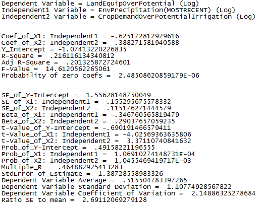
We use this new regression to estimate the portion of potentially irrigable land that is irrigated in the first year. The residual is then applied in every subsequent year as a multiplier.

Precipitation (EnvPrecipitation) changes each year as average annual precipitation changes due to total carbon in the atmosphere (a function of annual emissions from fossil fuels). Likewise, crop demand changes over time due to changes in demand in the component sectors (food, feed for livestock, food manufacturing/seeds, and industrial), along with changes in agricultural imports and exports, production, and loss. See the agricultural model documentation for a full description of our forecast for crop demand (Hughes & Rothman, 2014).

Utilization intensity of irrigated land (UIA)

There are four potential drivers of the UIA: increased competitiveness (irrigated land shrinks faster than equipped); land may be equipped to reduce drought risk (as a safeguard in bad years); limited water supply; and under poor economic conditions, areas equipped may not be maintained and become unusable (Wada et al., 2015).

We initialize utilization capacity using data from AQUASTAT. We use the most recent data point from the series described below. If there is no data available for a country, we use the global average of 77%. The utilization capacity remains constant over time.

SeriesLandIrActual%Equip

• Definition: Area equipped for irrigation: actually irrigated, %
• Source: AQUASTAT
• Units: Percent

Water requirement per unit of irrigated land (WRCI)

The water requirement per unit of irrigated land is the difference between total crop water requirements and the part supplied by precipitation. This is largely driven by the cropping intensity, or the ratio of harvested irrigated crop area over irrigated crop area (Fischer, Tubiello, van Velthuizen, & Wiberg, 2007; Wada et al., 2015).

Drivers of water requirements per unit of irrigated land

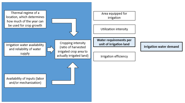
Water use per unit of irrigated land in IFs is estimated using a linear regression between agricultural water withdrawals (dependent variable) and irrigated land (independent variable). The details of the regression are shown below.

The regression used to forecast agricultural water demand uses the following data:

SeriesLandIrAreaEquip

• Definition: Area equipped for irrigation: total (1000 ha)
• Source: AQUASTAT
• Units: 1000 ha

SeriesLandIrActual%Equip

• Definition: Area equipped for irrigation: actually irrigated, %
• Source: AQUASTAT
• Units: Percent

SeriesWaterWithdAgriculture

• Definition: Agricultural water withdrawal
• Source: AQUASTAT
• Units: Cubic Km

We use a linear formulation for this regression. The results are shown below.

Regression used to forecast agricultural water demand

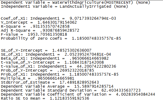
We use this regression to calculate the expected level of agricultural water demand (given land under irrigation) in the first year. This residual is then applied in every subsequent year as a multiplier.

Irrigation efficiency

The efficiency of irrigation can also change over time depending on the type of irrigation used and the technology behind it.

The model assumes that the efficiency of irrigation remains relatively constant over time for each country. We include a parameter on agricultural water demand however, that allows the user to adjust the efficiency of irrigation for countries, regions or the world.

Municipal water demand

Municipal (domestic) water demand is modelled in IFs by multiplying sectoral water intensity (municipal water demand per capita) by the size of the urban population. This is a similar formulation to other global water models like WaterGAP (Alcamo et al., 2003), H08 (Hanasaki et al., 2008; Shen, Oki, Utsumi, Kanae, & Hanasaki, 2008) and PCR-GLOBWB (Wada et al., 2016; Wada, Wisser, & Bierkens, 2014).

Per capita municipal water use increases as household incomes increase. As incomes increase, people adopt a more water-intensive lifestyle, which eventually saturates (Alcamo et al., 2003; Alcamo, Flörke, & Märker, 2007; Alcamo et al., 2007). The water sub-module of IFs uses GDP per capita and levels of access to piped water to forecast per capita municipal water use. To account for increased water use efficiency, the IFs model includes the percent of the population living in urban areas as an additional independent variable.

The dependent variable in the equation used to forecast municipal water demand is municipal water demand per capita:

${\frac {WATDEMAND_{municipal,r}}{POPURBAN}}$

We multiply this term by the size of the urban population (forecasted elsewhere) to get total municipal water demand.

$WATDEMAND_{municipal,r}={\frac {WATDEMAND_{municipal,r}}{POPURBAN}}*POPURBAN$

The independent variables for forecasting municipal water demand per capita are: GDP per capita (PPP); percent of the population living in urban areas; and the percentage of the population served with piped water.

Where municipal water demand per capita (WATDEMANDPC) is calculated using the following equation.

${\frac {WATDEMAND_{municipal,r}}{POPURBAN}}=x_{1}(ln(GDPPCP_{r}))+x_{2}(ln(WATSAFE_{piped,r}))-x_{3}(ln(UrbanPercentSmooth_{r}))$

Where GDPPCP represents GDP per capita at purchasing power parity (PPP), WATSAFE  represents the portion of the population with access to piped water and UrbanPercentSmooth represents the portion of the population living in urban areas but decreased for countries which are rapidly urbanizing. That is why there is a ‘smoothing’ of that variable for this equation. The coefficients of the first two independent variables (“$x_{1}$” and “$x_{2}$”) are positive—as when GDP per capita and access to piped water increase, water use per capita will also increase. The third coefficient “$x_{3}$” is negative because higher levels of urbanization are negatively correlated with water use per capita. All three of these independent variables are statistically significant at the global level.

While the portion of a country’s population living in urban areas is negatively correlated with water use per capita, the rate of urbanization is not necessarily negatively correlated with water use per capita. Countries with a large portion of their population living in urban areas might have water use efficiency infrastructure and policies in place, explaining the lower water use per capita. It takes time to put these water-conservation measures in place however.

For countries where the urbanization rate is greater than 1%:

$UrbanPercentSmooth_{r}=1.01*{\frac {(92-UrbanPercent_{r})^{.}75}{92}}$

This ensures that rapid urbanization does not lead to rapid water conservation. This is of particular concern for China, where IFs forecasts rapid urbanization over the next decades.

Municipal water use per capita (urban) increases in all income groups

Municipal water demand per capita for urban populations.

.

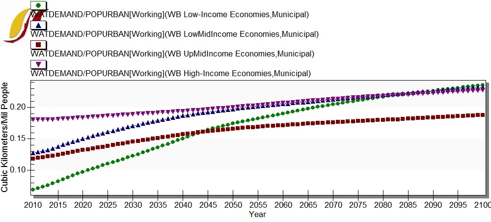
Industrial water demand

Industrial water demand is calculated as the sum of water demand for thermo-electric power generation (cooling) and water demand for the manufacturing sector.

Thermo-electric power generation

To forecast water consumption for thermo-electric power generation, we multiply total non-renewable electricity generation (in kWh) by a calculated value of water consumption per kWh. Water use per kWh is calculated as a function of both water scarcity within a country and the GDP per capita of the country. The more water-scarce a country is, the lower the desired water use per kWh. The actual water use per kWh is determined by this desired value together with the GDP per capita (PPP) of the country.

Water scarcity is calculated as the total water supply divided by the country’s population. This water-scarcity figure is then linearly mapped onto the range of [0.4 – 2.0]. This is a reasonable range for water use per kWh in a country (in terms of liters per kWh).

GDP per capita (PPP) for each country is linearly mapped onto the range [0-1] to calculate an ‘AbilityToAffordEfficiency’ variable.
Actual water use per unit of power generation (liters/kWh) is then calculated as:

$ActualWaterUsePerkWh_{r}=2-(AbilityToAffordElecEfficiency_{r}*(2-DesiredWaterUsePerkWh_{r}))$

This water use per kWh variable is then multiplied by non-renewable electricity generation to calculate total water consumption for electricity generation.

$IndustrialWaterDemandForElectricity_{r}=ActualWaterUsePerkWh_{r}*NonRenewablePowerGeneration_{r}$

Where NonRenewablePowerGeneration is calculated as:

$INFRAELECPROD_{r}-ElecRenew$

Where ElecRenew’ is calculated as

$(ENP_{renew,r}+ENP_{hydro,r})*1699.41*1000$

Renewable energy production is forecast in terms of billion barrels oil equivalent so the model must convert to gigawatt hours and then to kWh before it is subtracted from INFRAELECPROD. Industrial water demand for electricity is thus a function of non-renewable electricity generation, water scarcity, and GDP per capita (PPP).

Manufacturing

Although we do not have data on water demand for the manufacturing sector, using the calculations above for industrial water demand for electricity generation, we can estimate the portion of industrial water demand that is required for the manufacturing sector:

$IndustrialWaterDemand_{manufacturing,r}=WATDEMAND_{industrial,r}-IndustrialWaterDemand_{electricity,r}$

Manufacturing water withdrawal (km3) versus value added from the manufacturing sector (US$ billions).

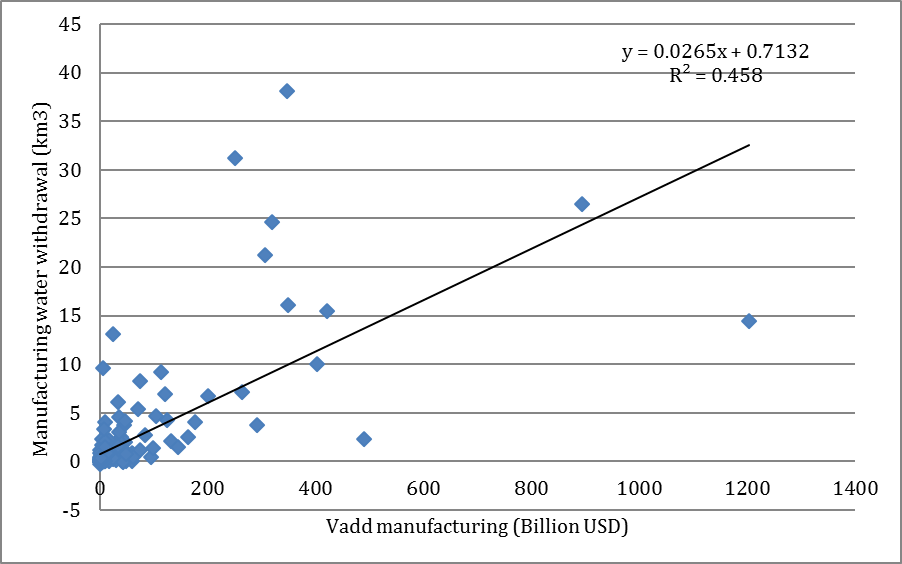
We use the size of a country’s manufacturing sector to drive industrial water demand for manufacturing. There is a correlation between this calculated industrial water demand for manufacturing and the size of the country’s manufacturing sector.

Industrial water demand for manufacturing is calculated by using the annual growth rate in the size of the manufacturing sector, adjusted by an elasticity of 0.45.

$IndustrialWaterDemand_{manufacturing,r,t}=IndustrialWaterDemand_{manufacturing,r,t-1}*({\frac {VADD_{manufacturing,r,t}}{VADD_{manufacturing,r,t-1}}})^{-.45}$

This elasticity figure (0.45) was calculated using country-specific elasticities between manufacturing value added growth rates and manufacturing water demand growth rates weighted by GDP:

${\frac {\sum _{r=1}^{AllCountries}{{\frac {log(ManufacturingWaterWithdrawalGR_{r})}{log(ManufacturingValueAddedGR_{r})}}*GDP_{r}}}{GlobalGDP}}$

Where ManufacturingWaterWithdrawalGR is the compound annual growth rate for industrial water demand for the manufacturing sector and ManufacturingValueAddedGR is the compound annual growth rate for value added from the manufacturing sector. We log both growth rates because the elasticity is calculated as an exponent rather than a multiplicative factor.

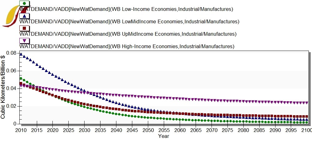
This new formulation means that industrial water use per unit of value added from the manufacturing sector decreases for all income groups.

Industrial water demand per unit (US$ billions) of value added from the manufacturing sector.

Using the equations described above, we calculate an “expected” water demand for each sector for each country. Using data from the pre-processor we are able to calculate residuals—the difference between the expected water demand and the actual water demand. $Residual_{r,s}=ExpectedWaterDemand_{r,s}-WATDEMAND_{r,s}$

These residuals do not change over time. We include efficiency parameters (waterefficiencym) on each of the water demand variables so that the user may decrease water demand in any sector.

Water demand is calculated the same way in all other years. We recalculate the expected level of water demand for each sector for each country using the driving variable, and then apply the residual. We also include the efficiency parameter multipliers in these calculations.

$WATDEMAND_{r,w}=(ExpectedWatDemand_{r,w}-Residual_{r,w})*\mathbf {waterefficiencym_{r,s}}$

Water supply

To model water supply in IFs we use the sum of surface water withdrawals, renewable groundwater withdrawals, non-renewable (fossil) groundwater withdrawal, treated and directly reused wastewater, and desalinated water. Treated wastewater that is not directly reused is added to surface water yield. This constitutes secondary water.

Surface water and renewable groundwater

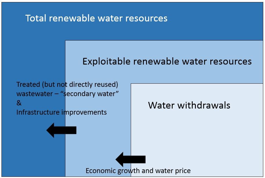
We use total renewable water resources as a constraint on exploitable renewable water resources (separated into surface water and groundwater) and exploitable renewable water resources as a constraint on water withdrawals. The diagram below shows the conceptual framework for forecasting surface water withdrawals. Withdrawals are driven by economic growth (GDP growth rate) and the water price index (described in section 3.5). Withdrawals are bound however, by the exploitable limit. Exploitable renewable surface water resources can increase due to “secondary water” – water that is treated but not directly reused. Exploitable surface water is bounded however, by the total renewable surface water.

Conceptual model for forecasting water withdrawals when withdrawals do not exceed exploitable limit.

We take our data for total renewable water resources, exploitable water resources, and water withdrawals from AQUASTAT. AQUASTAT defines total renewable water resources (TRWR) as, “The sum of internal renewable water resources (IRWR) and external renewable water resources (TRWR). It corresponds to the maximum theoretical yearly amount of water available for a country at a given moment” (FAO, 2016).

We use WATRESTOTALRENEW as a limit on the increase in WATRESEXPLOITRENEW. Exploitable water resources are usually a portion of total resources. This is because exploitable resources consider several restrictions on the use of water resources. The AQUASTAT data handbook defines these restrictions in terms of technical-economic criteria, environmental criteria, and geopolitical criteria.

AQUASTAT defines exploitable water resources as, “Exploitable water resources (also called manageable water resources or water development potential) are considered to be available for development, taking into consideration factors such as: the economic and environmental feasibility of storing floodwater behind dams, extracting groundwater, the physical possibility of storing water that naturally flows out to the sea, and minimum flow requirements (navigation, environmental services, aquatic life, etc). Methods to assess exploitable water resources vary from country to country” (FAO, 2016).

Exploitable water resources do however include secondary water so it can sometimes exceed total renewable water resources. This is rare but an important factor to keep in mind when forecasting. Thus, when we use total renewable resources as a limit on exploitable resources, we must remember to subtract secondary water from exploitable water resources first.

Since total renewable water resources does not account for the overlap between surface water and groundwater, we must recalculate total renewable water resources by subtracting this overlap. We then recalculate total renewable surface water and total renewable groundwater using this adjusted total.

$WATRESTOTALRENEW_{r,w}={\frac {WATRESTOTALRENEW_{r,w}}{WATRESTOTALRENEW(Overlap)}}*WATRESTOTALRENEW(NoOverlap)$

It is not possible, however, for exploitable water resources (excluding secondary water) to reach the TRWR limit. While exploitable water resources can increase, we assume that it cannot grow by more than 20%. We also assume that exploitable water resources cannot grow by more than .5% per year and that only one fortieth of remaining resources can be extracted in any year. Thus, the equation for exploitable water resources is:

$WATRESEXPLOITRENEW_{r,w}=$ $Min(WATRESEXPLOITRENEW_{t-1,w}*1.005,(({\frac {MaxExploitRenew_{w}-WATRESEXPLOITRENEW_{t-1,w}}{40}}))+WATRESEXPLOITRENEW_{t-1,w}))$

Where

$MaxExploitRenew_{w,r}=\mathbf {iwatresexploitrenew_{w,r}} *1.2$

iwatresexploitrenew is the exploitable renewable water resources in the first year. The subscript “w” represents that the variable is dimensioned in terms of surface and ground water. We also include a parameter, watresexploitrenewm on the total volume of exploitable water resources so that the user may increase or decrease this supply over time. After this growth rate is applied to exploitable surface water resources the secondary component is added to WATRESEXPLOITRENEW (surface). Secondary water is the total volume of treated wastewater that is not directly reused.

To forecast surface and groundwater withdrawals, we separate each country into one of two cases: countries where water withdrawals exceed the exploitable limit, and countries where water withdrawals do not exceed the exploitable limit. Surface water withdrawals and groundwater withdrawals are forecast separately. For example, a country can be overexploiting their surface water resources while groundwater withdrawals remain below the exploitable limit.

If surface water withdrawals are less than exploitable surface water resources, then surface water withdrawals are driven by a growth rate of 20 percent of the country’s latest GDP growth rate. This growth rate however cannot force surface water withdrawals to exceed one seventh of the remaining exploitable surface water (total exploitable surface water minus current surface water withdrawals).

The equation below describes the forecast equation for surface water withdrawals. It is calculated as the minimum of two terms: the previous year’s surface water withdrawals multiplied by 20 percent of the GDP growth rate of the country, and one seventh of the remaining exploitable potential plus the current level of withdrawal.

$WATERWITHDRAWAL_{r,surface,t+1}=$ $Min(WATERWITHDRAWAL_{r,surface,t}*1+0.2*IGDP_{r}),{\frac {RemainingPotentialExploitable}{7}}+WATERWITHDRAWAL_{r,surface,t})$

In the second case, where surface water withdrawals exceed the exploitable surface water limit, they are forced to converge to the exploitable limit over a 50-year time horizon. This time horizon is a parameter in the model (waterrenewconverge) that can be adjusted by the user.

$WATERWITHDRAWAL_{r,surface,t+1}=$ $WATERWITHDRAWAL_{r,surface,t}-({\frac {WATERWITHDRAWAL_{r,surface,t}-WATRESEXPLOITRENEW_{r,surface}}{\mathbf {waterrenewconverge} _{r,surface}}})$

Where waterrenewconverge is the 50-year default convergence time.

Conceptual model for forecasting water withdrawals when withdrawals exceed exploitable limit.

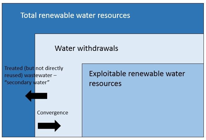
The exact same logic described above applies to groundwater withdrawals, and the parameter (waterrenewaconverge) is dimensioned by surface and groundwater. In the case of groundwater however, secondary water does not increase the exploitable limit – we assume treated wastewater that is not directly reused is released back into the system in the form of surface water.

If groundwater withdrawals are less than the exploitable limit:

$WATERWITHDRAWAL_{r,ground,t+1}=$ $Min(WATERWITHDRAWAL_{r,ground,t}*(1+0.2*IGDP_{r}),{\frac {RemainingPotentialExploitable}{7}}+WATERWITHDRAWAL_{r,ground,t})$

If groundwater withdrawals exceed the exploitable limit:

$WATERWITHDRAWAL_{r,ground,t+1}=$ $WATERWITHDRAWAL_{r,ground,t}-{\frac {WATERWITHDRAWAL_{r,ground,t}-WATRESEXPLOITRENEW_{r,ground}}{\mathbf {waterrenewconverge_{r,ground}} }}$

Both surface and groundwater withdrawals are adjusted based on the change in the water price index. A 0.5 elasticity is applied to the change in the water price index, which is then applied to both surface water withdrawals and groundwater withdrawals. Again, however, neither is permitted to grow faster than one seventh of the remaining exploitable potential.

$WATERWITHDRAWAL_{r,surface}=$ $Min(WATERWITHDRAWAL_{r,surface}*(1+(IncreaseInPrice*0.05)),$${\frac {WATERWITHDRAWAL_{r,surface}-WATRESEXPLOITRENEW_{r,surface}}{7}})+WATERWITHDRAWAL_{r,surface}$

The same logic and elasticity is applied to groundwater:

$WATERWITHDRAWAL_{r,ground}=$ $Min(WATERWITHDRAWAL_{r,ground}*(1+(IncreaseInPrice*0.05)),$${\frac {WATERWITHDRAWAL_{r,ground}-WATRESEXPLOITRENEW_{r,ground}}{7}})+WATERWITHDRAWAL_{r,ground}$

Wastewater

WASTEWATERSUPPLY is a multidimensional variable in the IFs model. The three dimensions are Produced, Treated, and TreatedAndReused. Most of our data on wastewater comes from the Aquastat database so we use their conceptual framework to model and forecast wastewater. Total produced wastewater is forecast in IFs as a portion of total municipal water demand. This relies on the assumption that wastewater that is reused among sectors comes primarily from collected municipal wastewater. Wastewater that is reused within a sector (for example, reuse of industrial wastewater within the same industrial factory) does not increase the water supply but, rather, decreases water demand in that particular sector.

Since we take the most recent data for each of these series they often do not reconcile. For example, treated wastewater may exceed produced wastewater, which is impossible. If a country’s volume of treated wastewater exceeds their supply of produced wastewater we assume that they treat 95% of their produced wastewater.

If we do not have data for a country’s volume of produced wastewater, we estimate this value using their municipal water demand. If we do not have data on the volume of treated wastewater, we estimate this value using a portion of their produced wastewater. The portion of a country’s produced wastewater that is treated is driven by GDP per capita. If we do not have data on the portion of treated wastewater that is directly reused, we estimate this value using a global average of 66%. Parameters are in IFs on both the portion of wastewater that is treated and the portion of treated wastewater that is directly reused: wastewaterportiontreated and wastewaterportiontreatedreused.

A portion of treated wastewater is directly reused and a portion of treated wastewater is discharged directly back into the water system. This discharge is considered “secondary water” and is added to exploitable surface water resources. Likewise, a portion of non-treated wastewater is directly re-used, usually by the agricultural sector, and a portion is discharged. The portion of non-treated wastewater that is not directly re-used is not added to exploitable surface water resources however. We do not yet have forecasts in IFs for the amount of non-treated wastewater that is directly reused. This is something that needs to be added to the model as some countries, like Mexico, use a large volume of non-treated municipal wastewater to irrigate crops.

Wastewater that is treated but not directly reused is then added to exploitable surface water resources.

$WATRESEXPLOITRENEW_{surface}=$$WATRESEXPLOITRENEW_{surface}+WASTEWATERSUPPLY_{treated}-WASTEWATERSUPPLY_{TreatedAndReused}$

Wastewater supply is calculated for all years using the same regressions described above for all years. The residuals for each of the equations do not change. The only way to increase supply of wastewater is to adjust municipal demand (which will affect total wastewater produced) or to adjust the wastewaterportiontreated parameter. This parameter is initialized as 1 but can be adjusted by the user. If the user does not change this parameter, the portion of produced wastewater that is treated will be driven by GDP per capita. If the user changes this to a value between 0 and 1 then that is the portion of produced wastewater that is treated.

If wastewaterportiontreated != 1 Then

$WASTEWATERSUPPLY_{treated,r}=WASTEWATER_{produced,r}*\mathbf {wastewaterportiontreated_{r}}$

Else

$WASTEWATERSUPPLY_{treated,r}=WASTEWATERSUPPLY_{produced,r}*TF(GDPPCP_{r})$

We use a log function of GDP per capita to forecast the portion of wastewater that is treated.

Treated wastewater is also affected by changes in the water price index, using a 0.5 elasticity. The equation below shows the water price index effect on treated wastewater. Treated wastewater is also bound by produced wastewater – a country cannot treat more wastewater than is produced.

$WASTEWATERSUPPLY_{r,treated,t+1}=$$Min(WASTEWATERSUPPLY_{r,produced},WASTEWATERSUPPLY_{r,treated,t}*(1+(IncreaseInPrice*0.05))$

3.2.3 Non-renewable (fossil) water withdrawals

We take fossil water resources data from 3 sources: FAO, UNESCO, and a peer-reviewed journal article from IOPScience. The IOP article however, does not differentiate between renewable groundwater resources and fossil groundwater resources so we subtract renewable groundwater resources from total fossil water resources.

For some countries, we have data on fossil water withdrawals but not fossil water resources. This creates problems in the forecast since future water withdrawals are based on remaining fossil water resources. For these countries, we estimate that their total fossil water resources are 10 times their current fossil water withdrawals.

$WATERRESFOSSIL=10*WATERWITHDRAWAL_{fossil}$

We model fossil water in IFs using a stock and flow dynamic. Total fossil water resources are used as a stock and fossil water withdrawal is the flow. Fossil water withdrawals increase at a one percent growth rate. This increase is bounded by the total supply of fossil water remaining. A country cannot extract more than one seventh of their remaining fossil water resources in any year. This number is taken from current fossil water extraction rates. The highest rate of extraction globally, occurring in the Nubian Sandstone Aquifer, is about one seventh of remaining resources.

$WATERWITHDRAWAL_{t+1,f}=$$Min(WATERWITHDRAWAL_{t,f}*1.01,{\frac {WATERRESFOSSIL}{7}})$

The subscript f represents fossil water.

3.2.4 Desalinated water

Desalinated water grows at an 8% growth rate, but this growth rate diminished over time. Desalinated water cannot decrease faster than 2% per year. Desalinated water increases based on an 8 percent growth rate (waterdesalinatedgr) which can be changed by the user. Growth in desalinated water is also adjusted based on the change in the water price index, using a 0.5 elasticity.

$WATERDESALINATED_{r,t+1}=$ $Min(WATERDESALINATED_{r,t}*(1+(IncreaseInPrice*0.05)),WASTERDESALINATED_{r,t}*(1+({\frac {\mathbf {waterdesalinated_{r}} }{100}})))$

Total water supply (WATERTOTALSUPPLY) is then calculated as the sum of these 5 water sources i.e. reused water, desalinated water, surface water, ground water, and fossil water.

$WATERTOTALSUPPLY=WASTEWATER_{TreatedAndReused}+DESALINATEDWATER+$ $WATERWITHDRAWAL_{Surface}+WASTERWITHDRAWAL_{Ground}+WATERWITHDRAWAL_{FossilGround}$

Because of the way we define water supply, demand can exceed supply of water resources. This usually means that the country is over exploiting their resources. This means that the country is using more surface water then their available yield, or withdrawing groundwater faster than the recharge rate. There are currently 23 countries that are over exploiting their water resources on a national level. It should be noted however, that since we are only looking at the national scale, local over-exploitation is not captured. This is particularly relevant to China and India—countries where over-exploitation is known to occur but not captured in our analysis. The top 5 countries in terms of national water exploitation are: Turkmenistan, Singapore, Egypt, Uzbekistan, and Syria, respectively.

While we do not forecast water withdrawal by source (surface, ground, and fossil ground), we have the data in IFs. This will be useful to forecast in the future so that we can determine the type over-exploitation that is occurring in water scarce countries.

We pull in data on surface water withdrawal, groundwater withdrawal, and total water withdrawal from Aquastat. Since total water withdrawal is the sum of surface water withdrawal and groundwater withdrawal, we can estimate surface water withdrawal if we have total water withdrawal and groundwater withdrawal. Likewise, if we have total water withdrawal and groundwater withdrawal we can estimate surface water withdrawal. Since, however, Aquastat does not differentiate between renewable groundwater withdrawal and fossil groundwater withdrawal we must first subtract fossil water withdrawal from groundwater withdrawal using other data.

$WATERWITHDRAWAL_{Ground}=$ $WATERWITHDRAWAL_{Ground}-WATERWITHDRAWAL_{FossilGround}$

If we have data on total water withdrawals but not surface water withdrawals and groundwater withdrawals then we estimate using global averages. We assume that 67% of a country’s water withdrawals come from surface water and 33% come from groundwater. If we do not have data on total water withdrawals we assume that a country’s total water withdrawals are equivalent to their total water demand. We then use the same global averages to determine which portion of this demand is met by surface water and which portion is met by groundwater. We do not yet reconcile total water demand with total water withdrawals, though, theoretically, they should be equivalent.

Water price index

The water price index is initialized at 100 in the first year of the model and changes year-to-year as a function of differences between supply and demand, using a proportional-integral-derivative controller (PID controller). The PID controller uses two terms to adjust the water price index: the integral or absolute distance of the system from the target, and the derivative, the change in value of the system from the previous year. In this case, the integral term is the absolute difference between the demand to supply ratio and 1 (the demand supply ratio in the first year) and the derivative term is the change in the demand to supply ratio from the previous year.

The following equation describes the four terms that are used by the PID controller to calculate the price index adjustment: the first term is the absolute change in the demand-supply ratio (the integral), the second term is the change in the demand-supply ratio from the previous year (the derivative), the third term is the impact that the integral has on the price index (0.3 but adjustable by user), and the fourth term is the impact that the derivative has on the price index (0.6 but adjustable by user).

$PriceAdjustment_{r}=PID(DemandSupplyRatio_{r,t}-1,(DemandSupplyRatio_{r,t}-DemandSupplyRatio_{r,t-1}),$ $ImpactofIntegralOnPrice,ImpactOfDerivativeonPrice)$

The change in the price index is then used to adjust water demand for each sector and water supply from each source.

Forward linkages

There is a switch (watertoyieldswitch) that can be set to 1, which allows water availability to impact agricultural yields.

$YL_{r}=YL_{r}*(1+({\frac {(adjustedWaterPerHA-waterPerHA)}{waterPerHA}}))^{waterToYieldElasticity}$

Where YL is agricultural yield, adjustedWaterPerHA is the agricultural water availability per HA of irrigated land after adjusting for the change in the price index, and waterPerHA is the agricultural water availability per HA of irrigated land before adjusting for the price index.

waterToYieldElasticity is set to 1.

Next steps

• Connect irrigated land to yield directly.
• Refine impact of water scarcity on yield.
• Include direct use of non-treated wastewater.
• More explicitly differentiate between “consumption” and “withdrawals”. Most other water models differentiate between the two (Wada et al., 2016).
• Include “livestock” as a sub-sector of agricultural water demand.
• Refine elasticities on demand and supply from price.

References

Hanasaki, N., Kanae, S., Oki, T., Masuda, K., Motoya, K., Shirakawa, N., … Tanaka, K. (2008). An integrated model for the assessment of global water resources–Part 2: Applications and assessments. Hydrology and Earth System Sciences, 12(4), 1027–1037.

Hughes, B. B., & Rothman, D. S. (2014). IFs Agriculture Model Documentation, Working paper 2014.04.28.

Neumann, K., Stehfest, E., Verburg, P. H., Siebert, S., Mueller, C., & Veldkamp, T. (2011). Exploring global irrigation patterns: A multilevel modelling approach. Agricultural Systems, 104(9), 703–713. https://doi.org/10.1016/j.agsy.2011.08.004

Riahi, K., van Vuuren, D. P., Kriegler, E., Edmonds, J., O’Neill, B. C., Fujimori, S., … Tavoni, M. (2017). The Shared Socioeconomic Pathways and their energy, land use, and greenhouse gas emissions implications: An overview. Global Environmental Change, 42, 153–168. https://doi.org/10.1016/j.gloenvcha.2016.05.009

Shen, Y., Oki, T., Utsumi, N., Kanae, S., & Hanasaki, N. (2008). Projection of future world water resources under SRES scenarios: water withdrawal / Projection des ressources en eau mondiales futures selon les scénarios du RSSE: prélèvement d’eau. Hydrological Sciences Journal, 53(1), 11–33. https://doi.org/10.1623/hysj.53.1.11

Wada, Y., Flörke, M., Hanasaki, N., Eisner, S., Fischer, G., Tramberend, S., … Wiberg, D. (2016). Modeling global water use for the 21st century: the Water Futures and Solutions (WFaS) initiative and its approaches. Geoscientific Model Development, 9(1), 175–222. https://doi.org/10.5194/gmd-9-175-2016

Wada, Y., Wisser, D., & Bierkens, M. F. P. (2014). Global modeling of withdrawal, allocation and consumptive use of surface water and groundwater resources. Earth System Dynamics, 5(1), 15–40. https://doi.org/10.5194/esd-5-15-2014