Revision as of 02:07, 20 August 2017

The most recent and complete agriculture model documentation is available on Pardee's website. Although the text in this interactive system is, for some IFs models, often significantly out of date, you may still find the basic description useful to you.

The IFs agricultural model tracks the supply and demand, including imports, exports, and prices, of three agricultural commodities: crops, meat, and fish. Crops, meat and fish have direct food, animal feed, industrial and food manufacturing uses. The agricultural model is also where land use dynamics and water use are tracked in IFs, as these are key resources for the agricultural sector.

The structure of the agriculture model is very much like that of the economic model. It combines a growth process with a partial economic equilibrium process using stocks and prices to seek a balance between the demand and supply sides. As in the economic model, no effort is made in the standard adjustment mechanism to obtain a precise equilibrium in any time step. Instead stocks serve as a temporary buffer and the model chases equilibrium over time.

The most important linkages between the agriculture model and other models within IFs are with the economic model. The economic model provides forecasts of average income levels, labor supply, total consumer spending, and agricultural investment, all of which are used in the agriculture model. In turn, the agriculture model provides forecasts on agricultural production, imports, exports, and demand for investment, which override the sectoral computations in the economic model. The agricultural model also has important links to the population and health models, using population forecasts and providing forecasts of calorie availability.

Dominant Relations

Agricultural production is a function of the availability of resources, e.g. land, livestock, capital, and labor, as well as climate factors and technology. Technology is most directly seen in the changing productivity of land in terms of crop yields, and in the production of meat relative to the input level of feed grain. The model also accounts for lost production (such as spoilage in the fields or in the first stages of the food supply chain), distribution and transformation losses and consumption losses (which account for food lost at the household levels) which are all determined by average income.

Agricultural demand depends on average incomes, prices, and a number of other factors. For example, changing diets can affect the demand for meat, which in turn affects the demand for feed crops. The industrial demand for crops, some of which is directed to the production of biofuels, is also affected by energy prices.

Production and demand, along with existing and desired stocks and historical trade patterns determine the trade in agricultural products. The differences in the supply of crops, meat, and fish (production after accounting for losses and trade) and the demand for these commodities are reflected in shifts in agricultural stocks. Stock shortages feed forward to actual consumption, which is addressed in the population model of IFs. Stocks, particularly changes in stocks, are a key driver of changes in crop prices. Crop prices are also influenced by the returns to agricultural investment and therefore to the basic underlying cost structure. Meat prices are tied to, and track world crop prices, while changes in fish prices are driven by changes in fish stocks.

Stocks and stock changes also play a role, along with general economic and agricultural demand growth, in driving the demand for agricultural investment. The actual levels of investment are finalized in the economic model of IFs and subject to constraints there. The investment can be of two types – investment for expanding and maintaining cropland (extensification) and investment for increasing crop yields per unit area (intensification). The expected relative rates of return determine the split.

The final key dynamics addressed in the agriculture model relate to land, livestock, and water. The latter of these is very straightforward, driven only by crop production. Changes in livestock are determined by changes in the amount of available grazing land, changes in the demand for meat, and the ability of countries to meet this demand as reflected in changing stocks.

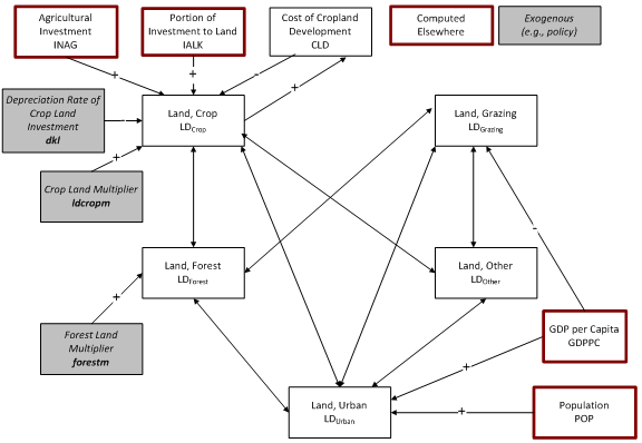
In the IFs model, land is divided into 5 categories: crop land, grazing land, forest land, ’other’ land, and urban or built-up land. First, changes in urban land are driven by changes in average income and population, and draws from all other land types. Second, the investment in cropland development is the primary driver of changes in cropland, with shifts being compensated by changes in forest and "other" land. Third, changes in grazing land are a function of average income, with shifts again being compensated by changes in forest and "other" land. Finally, conservation policies can influence the amount of forest land, with any necessary adjustments coming from crop and grazing land.

Structure and Agent System

System/Subsystem	Agriculture
Organizing Structure	Partial market equilibrium
Stocks	Capital, labor, accumulated technology, agricultural commodities, land
Flows	Production, loss, consumption, trade, investment
Key Aggregate Relationships (illustrative, not comprehensive)	Production function with endogenous technological change Price determination
Key Agent-Class Behavioral Relationships (illustrative, not comprehensive)	Household crop, meat, and fish consumption Industry crop use Livestock producers crop use

Flow Charts

Overview

The agriculture model combines a growth process in production with a partial equilibrium process that replaces the agricultural sector in the full-equilibrium economic model unless the user disconnects it. The model represents three agricultural commodities: crop, meat, and fish.

The key equilibrating variables are the stocks of the three commodities. Equilibration works via investment to control capital stock and via prices to control domestic demand.

Specifically, as food stocks rise, investment falls, restraining capital stock and agricultural production, and thus holding down stocks. Also, as stocks rise, prices fall, thereby increasing domestic demand, further holding down stocks. Domestic production and demand also influence imports and exports directly, which further affect stocks.

Agricultural Production

Crop Production

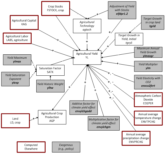
Crop production is most simply a product of the land under cultivation (cropland) and the crop yield per hectare of land. Yield is determined in a Cobb-Douglas type production function, the inputs to which are agricultural capital, labor, and technical change. Technical change is conceptualized as being responsive to price signals, but the model uses food stocks in the computation to enhance control over the temporal dynamics of responsiveness. Specifically, technology responds to the imbalance between desired and actual food stocks globally. In addition there is a direct response of yield change to domestic food stocks that represents not so much technical change as farmer behavior in the fact of market conditions (e.g. planting more intensively). Overall, basic annual yield growth is bound by the maximum of the initial model year's yield growth and an exogenous parameter of maximum growth.

This basic yield function is further subject to a saturation factor that is computed internally to the model̶–investments in increasing yield are subject to diminishing rather than constant returns to scale. Moreover, changes in atmospheric carbon dioxide (CO₂) will affect agricultural yields both directly through CO₂ and indirectly through changes in temperature and precipitation. Finally, the user can rely on parameters to increase or decrease yield patterns indirectly with a multiplier or to use parameters to control the saturation effect and the direct and indirect effects of CO₂ on crop yield.

Visual representation of agricultural yield

Meat and Fish Production

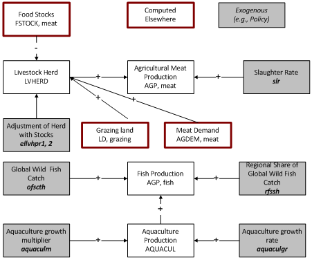
Meat and fish production are represented far more simply than crop production. Meat production is simply the product of livestock herd size and the slaughter rate. Meat production includes production of non-meat animal products (eg. Milk and eggs). The herd size changes over time in response to global and domestic meat stocks, as well as changes in the demand for meat and the amount of grazing land.

Fish production has two components: wild catch and aquaculture. The former is based on actual data and an exogenous parameter that allows the user to influence rate of catch. Aquaculture is assumed to continue to grow at a country-specific growth rate; a multiplier can also be used to increase or decrease aquaculture production.

Visual representation of meat and fish production

Agricultural Demand

Overview

Agricultural demand is divided into crops, meat, and fish. Crop demand is further divided into industrial, animal feed, and human food demand.

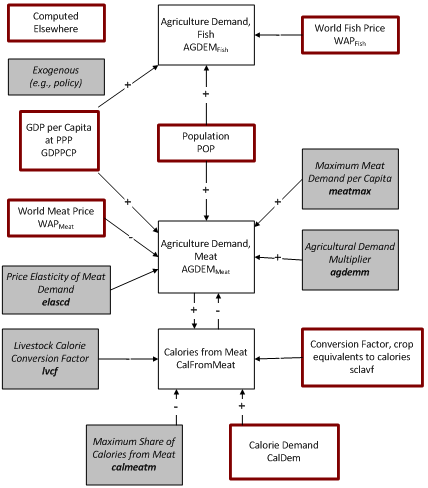
Food demand from crops, meat and fish are responsive to calorie demand, which in turn responds to GDP per capita (as a proxy for income). The division of calorie demand between demand for calories from crops and from meat and fish changes in response also to GDP per capita (increasing with income). Caloric demand is used as the basis to compute food demand through conversion to food demand in terms of grams per capita. The caloric value of demand is also used to compute food demand in terms of proteins per capita.

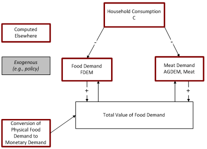
In addition to food demand, demand for feed, industrial demand for meat, crops and fish and food manufacturing demand are also computed. When all components of agricultural demand are computed, the price of the food elements of it are checked to assure that the total household demand for food does not exceed a high percentage of total country-level household consumption expenditures.

Calorie Demand

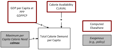
Crop use for food and meat demand are both influenced by calorie demand. Total per capita calorie demand is driven by GDP per capita, but can be limited by calorie availability as well as by an exogenous parameter specifying maximum calorie need.

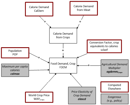
The calculations of demand for meat, fish and food crop determine the ultimate division of calorie sources. There is also a limit to the share of calories that can come from meat. The demand for calories from crops is simply the residual obtained by subtracting the demand for calories from meat and fish from the demand for total calories. Caloric value of demand is used to compute food demand in terms of grams per capita and in terms of proteins per capita. Caloric value of demand is adjusted for elasticities to prices for all three categories namely crops, meat and fish.

The user can manipulate calorie demand through the use of an exogenous calorie multiplier and can reduce undernourishment to 5 percent of the population over time through the usage of two other hunger elimination parameters.

Food Demand for Crops, Meat and Fish

Food demand is driven by the demand for calories. A conversion factor translates calorie demand into food demand in terms of grams per capita. Crop prices and an elasticity affect the resultant food demand. So too does a constraint on the maximum calories per capita and the size of the population.

Visual representation of animal feed demand for crops

Industrial Demand

Industrial demand (examples would be textile use of cotton or beverage inputs use of barley) is driven primarily by GDP per capita and population. Another important use in recent years has been for biofuels, and that demand component is responsive to world energy price and an elasticity.

Crop prices also influence total industrial demand for crops. A maximum per capita demand parameter constrains the total and an exogenous multiplier allows users to alter the total.

Visual representation of calorie demand

Feed Demand

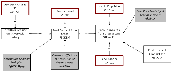
The total feed demand for the livestock herd is dependent on the weight of the livestock herd and per unit weight feed requirements. The per unit feed requirements increase with GDP per capita as populations move from meat sources such as chickens to more feed intensive ones such as pork and especially beef. But they also are reduced by change in the efficiency of converting feed to animal weight.

Some of the food requirements of livestock are met by grazing, thereby reducing the feed requirements. The feed equivalent of grazing depends on the amount of grazing land, the productivity of that land (computed in the initial year and highly variable across countries), and grazing intensity (which increases with crop prices).

Finally, the feed demand can be modified directly by an exogenous demand parameter that modifies industrial crop demand. The feed demand for meat and fish are calculated using ratios of the food demand to feed demand which are calculated in the initial years of the model. In addition to industrial demand and feed demand, food manufacturing demand is also calculated in the model on the basis of the food demand for all three categories (meat, crops and fish)

Visual representation of food demand for meat and fish

Total Agricultural Demand

Total Agricultural demand is the sum of demand for crops to serve industrial, animal feed, food manufacturing and human food purposes.

Visual representation of food demand for crops

Financial Constraint on Food Demand

Total food demand in million metric tons consists of the sum of crop demand, meat demand and food demand and fish demand. It can be, however, that the monetary value of those calculated demands is greater than the financial ability of households to pay for them. When that is the case, the food ,meat and fish demand are proportionately reduced.

Visual representation of financial constraint on food demand

Agricultural Investment and Capital

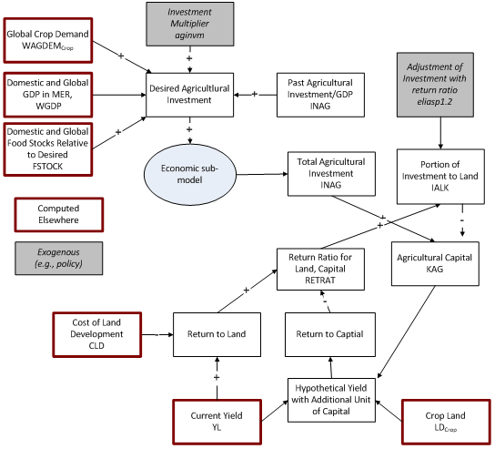
The level of total desired agricultural investment are driven by the rate of past investment as a portion of GDP, changes in global crop demand as a portion of GDP, and global crop stocks relative to desired levels. We have experimented also with tying investment to profit rates in agriculture, thereby linking it also to prices relative to costs. The user can use a multiplier to increase or decrease the desired level of investment. This desired amount of investment is passed to the economic model, where it must ‘compete’ with demands for investments in other sectors. The economic model returns a final investment level for use in agriculture.

Investment in agriculture has two possible targets. The first is capital stock. The second is land. The split between the two destinations is a function of the relative returns to cropland development and agricultural capital, the latter of which is determined by the increased yield that could be expected from an additional unit of agricultural capital.

Visual representation of agricultural investment and capital

Land Dynamics

In IFs, land use is divided into 5 categories: cropland, grazing land, forest land, "other" land, and urban or built-up land. Four key dynamics are involved in land use change. First, changes in urban land are driven by changes in average income and population, and draws from all other land types. Second, the investment in cropland development is the primary driver of changes in cropland, but this is also influenced by the cost of developing cropland, the depreciation rate, or maintenance cost, of cropland investment, and a user-controllable multiplier. The costs of developing cropland increase as the amount of cropland increases and, therefore, there is less other land available for conversion. Shifts in cropland are compensated by changes in forest and "other" land. Third, changes in grazing land are a function of average income, with shifts again being compensated by changes in forest and "other" land. Finally, conservation policies can influence the amount of forest land, with any necessary adjustments coming from crop and grazing land.

Visual representation of land dynamics

Agricultural Equations

Overview

Briefly, each year the agriculture model begins by estimating the production (pre- and post-production loss) of crops, meat, and fish. It then turns to the demand for these commodities. This begins with a computation of caloric demand from crops, meat, and fish, which is translated into demand for food going directly to consumers. Other demands for crops, meat, and fish are for feed, industrial uses (e.g. biofuels), and food manufacturing. Losses in the production, distribution and consumption of agricultural commodities are also accounted for. This is followed by computations for trade. The model then considers the balance between the demands and the available supply based on production, imports, and exports. Any excess supply increases stocks. In the case of excess demand, stocks are drawn down; this can result in shortages if there are not enough stocks, which leads to an inability to meet all of the demands. Levels of, and changes in, stocks influence prices for the coming year, as well as desired investment, which are passed to the economic model, which determines the actual amount of investment that will be available. With this knowledge, the model can then estimate values for changes in land development, agricultural capital, and livestock for the coming year.