Agriculture: Difference between revisions
StellahKwasi (talk | contribs) No edit summary |
StellahKwasi (talk | contribs) No edit summary |
||
| Line 610: | Line 610: | ||
---- | ---- | ||
<div> | <div> | ||
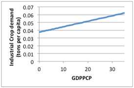
[file:///C:/Users/Ara/Desktop/Agricultural%20Documentation%20v19_AG.docx#_ftnref1 [1]] Equation is INDEM = 0.0376 + 0.000704 * GDPPCP | [file:///C:/Users/Ara/Desktop/Agricultural%20Documentation%20v19_AG.docx#_ftnref1 [1]] Equation is INDEM = 0.0376 + 0.000704 * GDPPCP | ||
== Final Agricultural Demand Adjustments in Forecast Years == | == Final Agricultural Demand Adjustments in Forecast Years == | ||
| Line 660: | Line 660: | ||
Finally, given the changes above, the total demand for crops is recalculated as the sum of the final values of feed, industry, and food demand. | Finally, given the changes above, the total demand for crops is recalculated as the sum of the final values of feed, industry, and food demand. | ||
[http://www.du.edu/ifs/help/media/images/ag-module/ageq55.png http://www.du.edu/ifs/help/media/images/ag-module/ageq55.png] | [http://www.du.edu/ifs/help/media/images/ag-module/ageq55.png http://www.du.edu/ifs/help/media/images/ag-module/ageq55.png] | ||
== Trade == | == Trade == | ||
| Line 764: | Line 764: | ||
Of course, the actual stock values (FSTOCK) are not allowed to go negative. If the basic stock level is negative, stocks are set at zero and a shortage (SHO) exists, which affects calorie availability. If the basic stock level is positive there is no shortage and stocks equal the basic level. | Of course, the actual stock values (FSTOCK) are not allowed to go negative. If the basic stock level is negative, stocks are set at zero and a shortage (SHO) exists, which affects calorie availability. If the basic stock level is positive there is no shortage and stocks equal the basic level. | ||
[http://www.du.edu/ifs/help/media/images/ag-module/ageq71.png http://www.du.edu/ifs/help/media/images/ag-module/ageq71.png] | [http://www.du.edu/ifs/help/media/images/ag-module/ageq71.png http://www.du.edu/ifs/help/media/images/ag-module/ageq71.png] | ||
== Calorie Availability == | == Calorie Availability == | ||
| Line 780: | Line 780: | ||
Calorie availability combines with regional calorie need in the population model for the calculation of possible starvation deaths (a seldom used variable because in official death statistics people do not die of starvation but rather of diseases associated with undernutrition); the population and health models therefore look instead to the impact of calorie availability on undernutrition and health. | Calorie availability combines with regional calorie need in the population model for the calculation of possible starvation deaths (a seldom used variable because in official death statistics people do not die of starvation but rather of diseases associated with undernutrition); the population and health models therefore look instead to the impact of calorie availability on undernutrition and health. | ||
[file:///C:/Users/Ara/Desktop/Agricultural%20Documentation%20v19_AG.docx#_ftnref1 [1]] Note this occurs in DATAPOP, not DATAAGRI. The historic data series is SERIESCalPCap. Missing data are estimated based on access to water and sanitation or average income. | [file:///C:/Users/Ara/Desktop/Agricultural%20Documentation%20v19_AG.docx#_ftnref1 [1]] Note this occurs in DATAPOP, not DATAAGRI. The historic data series is SERIESCalPCap. Missing data are estimated based on access to water and sanitation or average income. | ||
== Prices == | == Prices == | ||
| Line 808: | Line 808: | ||
The world price indices for crops and meat are computed, in the following year, as a weighted average of the domestic prices, with the weights given by crop and meat production: | The world price indices for crops and meat are computed, in the following year, as a weighted average of the domestic prices, with the weights given by crop and meat production: | ||
[http://www.du.edu/ifs/help/media/images/ag-module/ageq77.png http://www.du.edu/ifs/help/media/images/ag-module/ageq77.png] | [http://www.du.edu/ifs/help/media/images/ag-module/ageq77.png http://www.du.edu/ifs/help/media/images/ag-module/ageq77.png] | ||
== Returns and Profits == | == Returns and Profits == | ||
| Line 834: | Line 834: | ||
[http://www.du.edu/ifs/help/media/images/ag-module/ageq82.png http://www.du.edu/ifs/help/media/images/ag-module/ageq82.png] | [http://www.du.edu/ifs/help/media/images/ag-module/ageq82.png http://www.du.edu/ifs/help/media/images/ag-module/ageq82.png] | ||
A similar variable (wfprofitr) is calculated at the global level as a production weighted average of country/region values, but only for crops. | A similar variable (wfprofitr) is calculated at the global level as a production weighted average of country/region values, but only for crops. | ||
== Investment == | == Investment == | ||
| Line 958: | Line 958: | ||
[http://www.du.edu/ifs/help/media/images/ag-module/ageq103.png http://www.du.edu/ifs/help/media/images/ag-module/ageq103.png] | [http://www.du.edu/ifs/help/media/images/ag-module/ageq103.png http://www.du.edu/ifs/help/media/images/ag-module/ageq103.png] | ||
[file:///C:/Users/Ara/Desktop/Agricultural%20Documentation%20v19_AG.docx#_ftnref1 [1]]IFs does have a global parameter '''''agon'' ''' that can be used to break the link between the agriculture and economic model, in which case INAG is not overwritten. This is done by setting '''''agon'' ''' to a value less than 0.5. Doing so treats the agriculture model as a partial equilibrium model rather than a general equilibrium model. | [file:///C:/Users/Ara/Desktop/Agricultural%20Documentation%20v19_AG.docx#_ftnref1 [1]]IFs does have a global parameter '''''agon'' ''' that can be used to break the link between the agriculture and economic model, in which case INAG is not overwritten. This is done by setting '''''agon'' ''' to a value less than 0.5. Doing so treats the agriculture model as a partial equilibrium model rather than a general equilibrium model. | ||
== Land Dynamics == | == Land Dynamics == | ||
| Line 1,008: | Line 1,008: | ||
== Changes in Urban Land from Income and Population Changes == | == Changes in Urban Land from Income and Population Changes == | ||
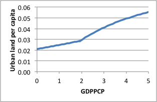
Changes in urban land result from changes in population and income. IFs first estimates a predicted level of urban land (LandUrbanPred), which is then compared to current urban land. Any changes are assumed to affect all other land types proportionately, unless this leads to not enough land in a particular category. The assumptions about the drivers of the predicted level of urban land differ somewhat between countrie[[File:Changes in Urban land from Y and population changes.png|right]]s depending upon their state of development, as measured by average income, in the base year. | Changes in urban land result from changes in population and income. IFs first estimates a predicted level of urban land (LandUrbanPred), which is then compared to current urban land. Any changes are assumed to affect all other land types proportionately, unless this leads to not enough land in a particular category. The assumptions about the drivers of the predicted level of urban land differ somewhat between countrie[[File:Changes in Urban land from Y and population changes.png|right|Changes in Urban land from Y and population changes.png]]s depending upon their state of development, as measured by average income, in the base year. | ||
For initially not as well off countries, GDPPCP in the base year < 5, the predicted level of urban land (LandUrbanPred) is estimated as a function of population and income growth. The growth with income is based on an estimated relationship between income and urban land per capita (landurbanr) summarized in the figure on the right<sup>[http://www.du.edu/ifs/help/understand/agriculture/equations/land/urban.html#footnote [1]] </sup>. | For initially not as well off countries, GDPPCP in the base year < 5, the predicted level of urban land (LandUrbanPred) is estimated as a function of population and income growth. The growth with income is based on an estimated relationship between income and urban land per capita (landurbanr) summarized in the figure on the right<sup>[http://www.du.edu/ifs/help/understand/agriculture/equations/land/urban.html#footnote [1]] </sup>. | ||
| Line 1,014: | Line 1,014: | ||
The predicted level of urban land (LandUrbanPred) is then given as | The predicted level of urban land (LandUrbanPred) is then given as | ||
http://www.du.edu/ifs/help/media/images/ag-module/ageq109.png | [http://www.du.edu/ifs/help/media/images/ag-module/ageq109.png http://www.du.edu/ifs/help/media/images/ag-module/ageq109.png] | ||
For initially well off countries, GDPPCP in the base year > 5, the predicted level of urban land is estimated as a function of population change. If population increases from the base year, is assumed to be same as urban land in the base year. If population declines from the base year, the predicted urban land area is estimated to decline, but only half as much as the population decline | For initially well off countries, GDPPCP in the base year > 5, the predicted level of urban land is estimated as a function of population change. If population increases from the base year, is assumed to be same as urban land in the base year. If population declines from the base year, the predicted urban land area is estimated to decline, but only half as much as the population decline | ||
http://www.du.edu/ifs/help/media/images/ag-module/ageq110.png | [http://www.du.edu/ifs/help/media/images/ag-module/ageq110.png http://www.du.edu/ifs/help/media/images/ag-module/ageq110.png] | ||
The change in urban land (NUrbLD) is then calculated as | The change in urban land (NUrbLD) is then calculated as | ||
http://www.du.edu/ifs/help/media/images/ag-module/ageq111.png | [http://www.du.edu/ifs/help/media/images/ag-module/ageq111.png http://www.du.edu/ifs/help/media/images/ag-module/ageq111.png] | ||
Limits are placed on the change in urban land area. First, if urban land is growing, the amount of increase in a single year cannot exceed 1/100<sup>th</sup> of a variable that is related to the change in the non-urban share of all other land from the base year (NonUrbanShrR) | Limits are placed on the change in urban land area. First, if urban land is growing, the amount of increase in a single year cannot exceed 1/100<sup>th</sup> of a variable that is related to the change in the non-urban share of all other land from the base year (NonUrbanShrR) | ||
http://www.du.edu/ifs/help/media/images/ag-module/ageq112.png | [http://www.du.edu/ifs/help/media/images/ag-module/ageq112.png http://www.du.edu/ifs/help/media/images/ag-module/ageq112.png] | ||
''where'' | ''where'' | ||
http://www.du.edu/ifs/help/media/images/ag-module/ageq113.png | [http://www.du.edu/ifs/help/media/images/ag-module/ageq113.png http://www.du.edu/ifs/help/media/images/ag-module/ageq113.png] | ||
Second, if urban land is declining, it is not permitted to fall below 10,000 hectares. Third, the changes are assumed to affect all other land categories proportionately. | Second, if urban land is declining, it is not permitted to fall below 10,000 hectares. Third, the changes are assumed to affect all other land categories proportionately. | ||
http://www.du.edu/ifs/help/media/images/ag-module/ageq114.png | [http://www.du.edu/ifs/help/media/images/ag-module/ageq114.png http://www.du.edu/ifs/help/media/images/ag-module/ageq114.png] | ||
However, this is not allowed to result in the area for a given land category falling below 1,000 hectares. Thus, there may be a slight reduction in the amount of new urban land in certain cases. | However, this is not allowed to result in the area for a given land category falling below 1,000 hectares. Thus, there may be a slight reduction in the amount of new urban land in certain cases. | ||
| Line 1,041: | Line 1,041: | ||
<div> | <div> | ||
[file:///C:/Users/Ara/Desktop/Agricultural%20Documentation%20v19_AG.docx#_ftnref1 [1]] Equation is Urban land per Capita = 0.021 + 0.0039*GDPPCP when GDPPCP < 1.92 in the base year and Urban land per Capita = 0.01 + 0.0283*ln(GDPPCP) when GDPPCP >= 1.92 in the base year. | [file:///C:/Users/Ara/Desktop/Agricultural%20Documentation%20v19_AG.docx#_ftnref1 [1]] Equation is Urban land per Capita = 0.021 + 0.0039*GDPPCP when GDPPCP < 1.92 in the base year and Urban land per Capita = 0.01 + 0.0283*ln(GDPPCP) when GDPPCP >= 1.92 in the base year. | ||
</div> | </div><header><hgroup> | ||
== Changes in Cropland due to Investment and/or Depreciation == | == Changes in Cropland due to Investment and/or Depreciation == | ||
The changes in cropland are driven by the economics of land. Specifically, they are a function of the profitability of cropland. Also, they are assumed to affect, at least directly, only the forest and the other land categories. | </hgroup></header> The changes in cropland are driven by the economics of land. Specifically, they are a function of the profitability of cropland. Also, they are assumed to affect, at least directly, only the forest and the other land categories. | ||
A maximum amount of cropland expansion each year (MaxLandExpansion) is fixed by the amount of forest land, the amount of other lands, the amount of potential arable land, and the existing amount of cropland. The maximum amount of expansion must be at least 2/100<sup>th</sup> of the existing cropland, but beyond that it cannot exceed either the total amount of forest and other land or the difference between 110% of the potential arable land (landarablepot) and current cropland. | A maximum amount of cropland expansion each year (MaxLandExpansion) is fixed by the amount of forest land, the amount of other lands, the amount of potential arable land, and the existing amount of cropland. The maximum amount of expansion must be at least 2/100<sup>th</sup> of the existing cropland, but beyond that it cannot exceed either the total amount of forest and other land or the difference between 110% of the potential arable land (landarablepot) and current cropland. | ||
| Line 1,052: | Line 1,052: | ||
If neither of the conditions mentioned in the previous paragraph is met, i.e., if the country is not too wealthy and there is an ‘adequate’ amount of land for expanding cropland, the amount of change in cropland (lddev) is initially calculated as | If neither of the conditions mentioned in the previous paragraph is met, i.e., if the country is not too wealthy and there is an ‘adequate’ amount of land for expanding cropland, the amount of change in cropland (lddev) is initially calculated as | ||
http://www.du.edu/ifs/help/media/images/ag-module/ageq115.png | [http://www.du.edu/ifs/help/media/images/ag-module/ageq115.png http://www.du.edu/ifs/help/media/images/ag-module/ageq115.png] | ||
''where'' | ''where'' | ||
| Line 1,068: | Line 1,068: | ||
Note that this equation takes into account the need to maintain existing cropland. Also, at this point, the value of lddev is bound from below to ensure that it does not imply a greater than 10 percent decrease in existing cropland. For relatively poor countries (GDPPCP < 10), the constraint is even stricter. Specifically, IFs calls for a shift in funds to ensure that no cropland is lost. The desired shift in funds is given as | Note that this equation takes into account the need to maintain existing cropland. Also, at this point, the value of lddev is bound from below to ensure that it does not imply a greater than 10 percent decrease in existing cropland. For relatively poor countries (GDPPCP < 10), the constraint is even stricter. Specifically, IFs calls for a shift in funds to ensure that no cropland is lost. The desired shift in funds is given as | ||
http://www.du.edu/ifs/help/media/images/ag-module/ageq116.png | [http://www.du.edu/ifs/help/media/images/ag-module/ageq116.png http://www.du.edu/ifs/help/media/images/ag-module/ageq116.png] | ||
The actual shift in funds is limited to 90 percent of the available funds, however, where the available funds are the investment in agriculture not initially designated for cropland development | The actual shift in funds is limited to 90 percent of the available funds, however, where the available funds are the investment in agriculture not initially designated for cropland development | ||
http://www.du.edu/ifs/help/media/images/ag-module/ageq117.png | [http://www.du.edu/ifs/help/media/images/ag-module/ageq117.png http://www.du.edu/ifs/help/media/images/ag-module/ageq117.png] | ||
The value of lddev given the actual shift in funds is given as | The value of lddev given the actual shift in funds is given as | ||
http://www.du.edu/ifs/help/media/images/ag-module/ageq118.png | [http://www.du.edu/ifs/help/media/images/ag-module/ageq118.png http://www.du.edu/ifs/help/media/images/ag-module/ageq118.png] | ||
In addition, the share of investment in agriculture designated for cropland development is updated to be<sup>[http://www.du.edu/ifs/help/understand/agriculture/equations/land/crop.html#footnote [1]]</sup> | In addition, the share of investment in agriculture designated for cropland development is updated to be<sup>[http://www.du.edu/ifs/help/understand/agriculture/equations/land/crop.html#footnote [1]]</sup> | ||
<div>http://www.du.edu/ifs/help/media/images/ag-module/ageq119.png</div><div> | <div>[http://www.du.edu/ifs/help/media/images/ag-module/ageq119.png http://www.du.edu/ifs/help/media/images/ag-module/ageq119.png]</div><div> | ||
The changes in cropland are linked to changes in land in the forest and ‘other’ categories. The amount coming from/going to forests reflects the share of forest land relative to ‘other’ land, as well as the current level of development | The changes in cropland are linked to changes in land in the forest and ‘other’ categories. The amount coming from/going to forests reflects the share of forest land relative to ‘other’ land, as well as the current level of development | ||
http://www.du.edu/ifs/help/media/images/ag-module/ageq120.png | [http://www.du.edu/ifs/help/media/images/ag-module/ageq120.png http://www.du.edu/ifs/help/media/images/ag-module/ageq120.png] | ||
''where'' | ''where'' | ||
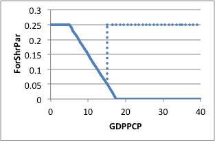
ForShrPar is given by the function depicted below that | ForShrPar is given by the function depicted below that | ||
[[File:Changes in cropland due to Investment and or Depreciation.png|center]] | |||
<div> | |||
The solid line holds when land is being converted from forests to cropland (lddev > 0) and the dotted line holds when land is being converted from cropland to forests (lddev < 0). In either case, this implies that the less of the change is related to forest land than would be expected by its share. Two other qualifiers are that the changes in forest land (LDDEVFor) and the changes in ‘other’ land cannot exceed 90 percent of existing land in these categories and the shifts cannot result in either land category falling below 1,000 hectares. These limits feedback to the change in cropland, finally resulting in the following | |||
http://www.du.edu/ifs/help/media/images/ag-module/ageq121.png | |||
http://www.du.edu/ifs/help/media/images/ag-module/ageq122.png | |||
http://www.du.edu/ifs/help/media/images/ag-module/ageq123.png | |||
http://www.du.edu/ifs/help/media/images/ag-module/ageq124.png | |||
Turning back to the future cost of cropland development, this is estimated differently based only on whether there is ‘adequate’ room for cropland land expansion, defined as when the maximum amount of cropland expansion is greater than 10 percent of existing cropland. If this is the case, the future price of cropland is estimated as | |||
http://www.du.edu/ifs/help/media/images/ag-module/ageq125.png | |||
''where'' | |||
RemRat is the ratio of the maximum land for expansion in the first year to the maximum land for expansion in the current year, with a maximum value of 10 | |||
http://www.du.edu/ifs/help/media/images/ag-module/ageq126.png | |||
This basically states that the price of cropland development grows linearly with growth in cropland and exponentially with declines in available land for cropland expansion. | |||
Alternatively, if the maximum amount of cropland expansion in a given year is less than or equal to10 percent of existing cropland, the cost of bringing new land under cultivation is assumed to grow at the maximum of either 2 percent per year from the cost in the first year or the growth of cropland from the first year. Furthermore, it is not allowed to decline. Thus, | |||
http://www.du.edu/ifs/help/media/images/ag-module/ageq127.png | |||
</div> | |||
---- | |||
<div> | |||
[file:///C:/Users/Ara/Desktop/Agricultural%20Documentation%20v19_AG.docx#_ftnref1 [1]] Given that IALK represents a share value, it is also bound to be <= 1. | |||
</div> <header><hgroup> | |||
== Changes in Grazing Land == | |||
</hgroup></header> | |||
IFs assumes that relatively poor countries (GDPPCP < 10) will continue to develop additional grazing land, whereas relatively rich countries (GDPPCP > 15) will retire grazing land. No change is expected in countries with average income between $10,000 and $15,000. The annual expansion of grazing land in poor countries is initially estimated as 0.5 percent of the amount of grazing land in the first year. The retirement of grazing land in richer countries is initially estimated as 0.2 percent of current grazing land. | |||
As with cropland, any changes in grazing land will be compensated by changes in forest and ‘other’ land. Each category is initially assumed to be affected proportionately, e.g., | |||
http://www.du.edu/ifs/help/media/images/ag-module/ageq127.png | |||
Unlike the case for changes in cropland, there is no adjustment to the forest share as a function of income or the direction of change in grazing land. As with the changes in cropland, however, the changes in forest and ‘other’ land cannot exceed 90 percent of existing land in these categories and the shifts cannot result in either land category falling below 1,000 hectares. Again, these limits feed back to the change in grazing land. | |||
<header><hgroup> | |||
== Change in Forest Land due to a Policy Choice == | |||
</hgroup></header> | |||
The model user can also force the land in forest area to increase or decrease at the expense of crop and grazing land via a forest multiplier '''''forestm'' '''. The change in forestland, LDSHIFT, is bound. In the case of an increase, i.e., '''''forestm'' ''' > 1, the amount of added land is limited to 20 percent of crop and grazing land; in the case of a decrease, i.e., '''''forestm'' ''' < 1, the amount of forest land removed is limited to 20 percent of existing forest land. | |||
http://www.du.edu/ifs/help/media/images/ag-module/ageq128.png | |||
http://www.du.edu/ifs/help/media/images/ag-module/ageq129.png | |||
The amount of land taken from cropland and grazing land is proportional to the amount of each. | |||
http://www.du.edu/ifs/help/media/images/ag-module/ageq130.png | |||
http://www.du.edu/ifs/help/media/images/ag-module/ageq131.png | |||
http://www.du.edu/ifs/help/media/images/ag-module/ageq132.png | |||
<header><hgroup> | |||
== Final Checks and Renormalization of Land Use == | |||
</hgroup></header> | |||
Two final adjustments are made to the land area values to clean up any quirks that might have be introduced in the previous processes. First, the values for each category are bound between one thousand and ten billion hectares. Second, the values are normalized so that the sum of the categories equals the total amount of land. | |||
http://www.du.edu/ifs/help/media/images/ag-module/ageq133.png | |||
Finally, a value for world forest area (WFORST) is calculated at the end of this process by summing forestland area across all countries. | |||
http://www.du.edu/ifs/help/media/images/ag-module/ageq134.png | |||
<header><hgroup> | |||
== Livestock Dynamics == | |||
</hgroup></header> | |||
In addition to capital and land, the other "stock" or "level" variable with important temporal dynamics is the livestock herd (LVHERD). The size of the herd size (LVHERD) in the first year is calculated simply as the base year value of meat production divided by the slaughter rate, '''''slr'' '''.<sup>[http://www.du.edu/ifs/help/understand/agriculture/equations/livestock.html#footnote [1]]</sup> | |||
The growth of the herd size in future years is driven by changes in meat demand at both the national and global levels, changes in meat stocks at both the national and global levels, and changes in grazing land at the national level. | |||
At the national level, herd sizes for the next year are first estimated as a function of changes in national meat demand, national meat stocks, national grazing land, and an adjustment factor related to national meat stocks: | |||
http://www.du.edu/ifs/help/media/images/ag-module/ageq135.png | |||
The forecasts of meat demand (AGDEM<sub>r,f=2</sub>) and grazing land (LD<sub>r,l=2</sub>) are described in the [http://www.du.edu/ifs/help/understand/agriculture/equations/demand/meat.html Meat Demand] section and the [http://www.du.edu/ifs/help/understand/agriculture/equations/land/grazing.html Changes in Grazing Land] section, respectively. The national stock adjustment factors are calculated using the same ADJSTR function as used to adjust crop yields. In this case, the desired stock level is given as agdstltimes the sum of national meat demand (AGDEM<sub>r,f=2</sub>) and national meat production (AGP<sub>r,f=2</sub>). As mentioned previously, agdstl is set to be 1.5 times '''''dstl'' ''', which is a global parameter that can be adjusted by the user. Also, the two parameters that determine how much of an adjustment there is due to changes in stock levels from the previous years and the difference between the actual and desired stock levels are hard coded with values of -0.05 and -0.1, respectively. | |||
At the global level, herd sizes for the next year are estimated as a function of changes in global meat demand, global meat stocks, and an adjustment factor related to global meat stocks: | |||
<div> | |||
http://www.du.edu/ifs/help/media/images/ag-module/ageq136.png | |||
</div> | |||
<span>The global stock adjustment factor is calculated in the same manner as the national stock adjustment factors, only using global values for actual and desired stocks.</span> | |||
<span>Finally, the herd sizes for the next year are normalized so that the sum of the national values equals the global value:</span> | |||
http://www.du.edu/ifs/help/media/images/ag-module/ageq137.png | |||
[file:///C:/Users/Ara/Desktop/Agricultural%20Documentation%20v19_AG.docx#_ftnref1 [1]] For details on the base year value of meat production, which is based on historical data related to production, imports, exports, and assumptions about expected meat consumption and production losses, see the description of agricultural data initialization in the pre-processor. | |||
<header><hgroup> | |||
== Water Dynamics == | |||
</hgroup></header> | |||
<span>Water use begins with data on total water withdrawals from FAO Aquastat. These are divided by the size of the population to get an estimate of water use per capita.</span> | |||
<span>In future years, water use per capita is forecast to increase in parallel with crop production per capita. Specifically, an expected level of water use per capita as a function of crop production per capita (see figure below) is calculated for crop production in the current year (CropPC) and crop production in the first year (CropPCI). The ratio of these values is multiplied by the water use per capita in the first year (WatUsePCI) to get water use per capita in the current year (WatUsePC). This is multiplied by population (POP) to get total water use (WATUSE).</span> | |||
http://www.du.edu/ifs/help/media/images/ag-module/ageq138.png | |||
http://www.du.edu/ifs/help/media/images/ag-module/ageq139.png | |||
</div></div></div></div></div></div></div></div></div></div></div></div></div></div></div></div><br/></div></div><br/> | </div></div></div></div></div></div></div></div></div></div></div></div></div></div></div></div><br/></div></div><br/> | ||
== == | == == | ||
Revision as of 21:42, 7 January 2017
The most recent and complete agriculture model documentation is available on Pardee's website. Although the text in this interactive system is, for some IFs models, often significantly out of date, you may still find the basic description useful to you.
The IFs agriculture model tracks the supply and demand, including imports, exports, and prices, of three agricultural commodities: crops, meat, and fish. Crops have direct food, animal feed, and industrial uses. Meat and fish have only food use. The agriculture model is also where land use dynamics and water use are tracked in IFs, as these are key resources for the agricultural sector.
The structure of the agriculture model is very much like that of the economic model. It combines a growth process with a partial economic equilibrium process using stocks and prices to seek a balance between the demand and supply sides. As in the economic model, no effort is made in the standard adjustment mechanism to obtain a precise equilibrium in any time step. Instead stocks serve as a temporary buffer and the model chases equilibrium over time.
The most important linkages between the agriculture model and other models within IFs are with the economic model. The economic model provides forecasts of average income levels, labor supply, total consumer spending, and agricultural investment, as well as parameters such as the capital elasticity of substitution, all of which are used in the agriculture model. In turn, the agriculture model provides forecasts on agricultural production, imports, exports, and demand for investment, which override the sectoral computations in the economic model. The agriculture model also has important links to the population and health models, using population forecasts and providing forecasts of calorie availability.
Structure and Agent System: Agriculture
System/Subsystem
|
Agriculture
|
Organizing Structure
|
Partial market equilibrium
|
Stocks
|
Capital, labor, accumulated technology, agricultural commodities, land
|
Flows
|
Production, loss, consumption, trade, investment
|
Key Aggregate Relationships (illustrative, not comprehensive)
|
Production function with endogenous technological change Price determination |
Key Agent-Class Behavior Relationships (illustrative, not comprehensive)
|
Household crop, meat, and fish consumption Industry crop use Livestock producers crop use |
Dominant Relations: Agriculture
Agricultural production is a function of the availability of resources, e.g. land, livestock, capital, and labor, as well as climate factors and technology. Technology is most directly seen in the changing productivity of land in terms of crop yields, and in the production of meat relative to the input level of feed grain. The model also accounts for lost production (such as spoilage in the fields or in the food supply chain), which is determined by average income.
Agricultural demand depends on average incomes, prices, and a number of other factors. For example, changing diets can affect the demand for meat, which in turn affects the demand for feed crops. The industrial demand for crops, some of which is directed to the production of biofuels, is also affected by energy prices.
Production and demand, along with existing and desired stocks and historical trade patterns determine the trade in agricultural products. The differences in the supply of crops, meat, and fish (production after accounting for losses and trade) and the demand for these commodities are reflected in shifts in agricultural stocks. Stock shortages feed forward to actual consumption, which is addressed in the population model of IFs. Stocks, particularly changes in stocks, are a key driver of changes in crop prices. Crop prices are also influenced by the returns to agricultural investment and therefore to the basic underlying cost structure. Meat prices are tie to, and track crop prices, while changes in fish prices are driven by changes in fish stocks.
Stocks and stock changes also play a role, along with general economic and agricultural demand growth, in driving the demand for agricultural investment. The actual levels of investment are finalized in the economic model of IFs and subject to constraints there. The investment can be of two types – investment for expanding and maintaining cropland (extensification) and investment for increasing crop yields per unit area (intensification). The expected relative rates of return determine the split.
The final key dynamics addressed in the agriculture model relate to land, livestock, and water. The latter of these is very straightforward, driven only by crop production. Changes in livestock are determined by changes in the amount of available grazing land, changes in the demand for meat, and the ability of countries to meet this demand as reflected in changing stocks.
In the IFs model, land is divided into 5 categories: crop land, grazing land, forest land, ’other’ land, and urban or built-up land. First, changes in urban land are driven by changes in average income and population, and draws from all other land types. Second, the investment in cropland development is the primary driver of changes in cropland, with shifts being compensated by changes in forest and "other" land. Third, changes in grazing land are a function of average income, with shifts again being compensated by changes in forest and "other" land. Finally, conservation policies can influence the amount of forest land, with any necessary adjustments coming from crop and grazing land.
Agriculture Flow Charts
Overview
The agriculture model combines a growth process in production with a partial equilibrium process that replaces the agricultural sector in the full-equilibrium economic model unless the user disconnects it. The model represents three agricultural commodities: crop, meat, and fish.
The key equilibrating variables are the stocks of the three commodities. Equilibration works via investment to control capital stock and via prices to control domestic demand.
Specifically, as food stocks rise, investment falls, restraining capital stock and agricultural production, and thus holding down stocks. Also, as stocks rise, prices fall, thereby increasing domestic demand, further holding down stocks. Domestic production and demand also influence imports and exports directly, which further affect stocks.
This section presents several block diagrams that provide an overview of the variables and dynamics of the agricultural model.
Agricultural Production
Crop Production
Crop production is most simply a product of the land under cultivation (cropland)
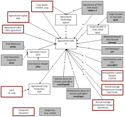
and the crop yield per hectare of land. Yield is determined in a Cobb-Douglas type production function, the inputs to which are agricultural capital, labor, and technical change. Technical change is conceptualized as being responsive to price signals, but the model uses food stocks in the computation to enhance control over the temporal dynamics of responsiveness. Specifically, technology responds to the imbalance between desired and actual food stocks globally. In addition there is a direct response of yield change to domestic food stocks that represents not so much technical change as farmer behavior in the fact of market conditions (e.g. planting more intensively). Overall, basic annual yield growth is bound by the maximum of the initial model year's yield growth and an exogenous parameter of maximum growth.
This basic yield function is further subject to a saturation factor that is computed internally to the model̶–investments in increasing yield are subject to diminishing rather than constant returns to scale. Moreover, changes in atmospheric carbon dioxide (CO2) will affect agricultural yields both directly through CO2 and indirectly through changes in temperature and precipitation. Finally, the user can rely on parameters to increase or decrease yield patterns indirectly with a multiplier or to use parameters to control the saturation effect and the direct and indirect effects of CO2 on crop yield.
Meat and Fish Production
Meat and fish production are represented far more simply than crop p
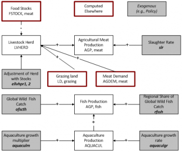
roduction. Meat production is simply the product of livestock herd size and the slaughter rate. The herd size changes over time in response to global and domestic meat stocks, as well as changes in the demand for meat and the amount of grazing land.
Fish production has two components: wild catch and aquaculture. The former is based on global catch and the regional share, both of which are specified exogenously. Aquaculture is assumed to continue to grow at a country-specific growth rate; a multiplier can also be used to increase or decrease aquaculture production.
Agricultural Demand
Overview
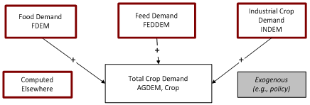
Agricultural demand is divided into crops, meat, and fish. Crop demand is further divided into industrial, animal feed, and human food demand.
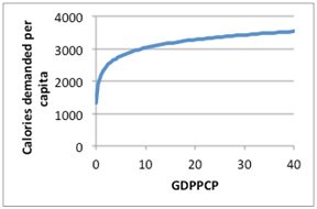
Meat and food demand are responsive to calorie demand, which in turn responds to GDP per capita (as a proxy for income). The division of calorie demand between demand for calories from crops and from meat changes in response also to GDP per capita (increasing with income).
When all components of agricultural demand are computed, the price of the food elements of it are checked to assure that the total household demand for food does not exceed a high percentage of total country-level household consumption expenditures.
Industrial Crop Demand
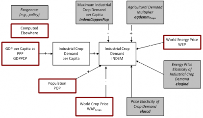
Industrial crop demand (examples would be textile use of cotton or beverage inputs use of barley) is driven primarily by GDP per capita and population. Another important use in recent years has been for
biofuels, and that demand component is responsive to world energy price and an elasticity.
Crop prices also influence total industrial agricultural demand. A maximum per capita demand parameter constrains the total and an exogenous multiplier allows users to alter the total.
Animal Feed Demand for Crops
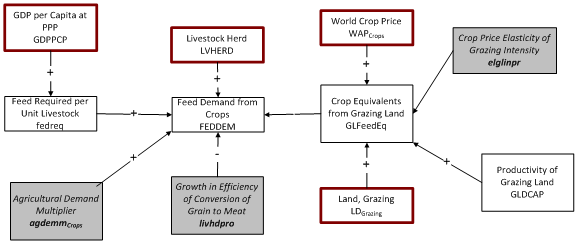
The total feed demand for the livestock herd is dependent on the weight of the livestock herd and the per weight unit feed requirements. The per unit feed requirements increase with GDP per capita as populations move from meat sources such as chickens to more feed intensive ones such as pork and especially beef. But they also are reduced by change in the efficiency of converting feed to animal weight.
Some of the food requirements of livestock are met by grazing, thereby reducing the feed requirements. The feed equivalent of grazing depends on the amount of grazing land, the productivity of that land (computed in the initial year and highly variable across countries), and grazing intensity (which increases with crop prices).
Finally, the feed demand can be modified directly by the same exogenous crop demand parameter that modifies industrial crop demand.
Calorie Demand
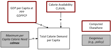
Crop use for food and meat demand are both influenced by calorie demand. Total per capita calorie demand is driven by GDP per capita, but can be limited by calorie availability as well as by an exogenous parameter specifying maximum calorie need.
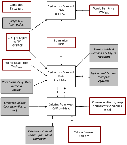
The calculations of demand for meat and food crop determine the ultimate division of calorie sources (shown in other topics). Calories from meat are connected to the demand for meat in tons, with adjustments for the conversion of meat to crop equivalents and then crop equivalents to calories. There is also a limit to the share of calories that can come from meat. The demand for calories from crops is simply the residual obtained by subtracting the demand for calories from meat from the demand for total calories.
Food Demand for Meat and Fish
Meat and fish demand are only for food. Fish demand is the simpler. It is driven by changes in population, GDP per capita, and fish prices (the elasticity of demand for prices is currently hard-coded in the model and should be made a parameter).
The demand for meat also increases with population and GDP per capita, and falls with increasing meat prices. Additionally, it is also subject to a maximum level per capita. Further it is subject to a constraint that the calories provided by meat cannot exceed an exogenously specified maximum share of total calorie demand; if it does upon first calculation, it is recalculated to be consistent with that share. Finally, meat demand can be modified with a multiplier.
Food Demand for Crops
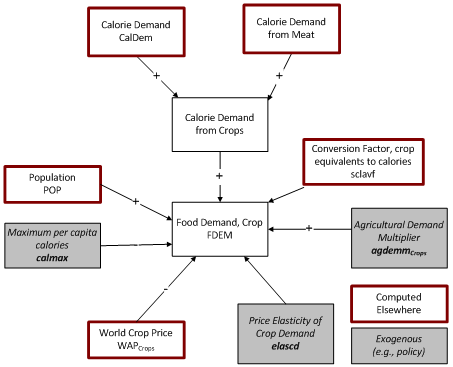
Food demand is driven by the demand for calories from crops, which is the residual of the total calorie demand and the demand for meat. A conversion factor translates calorie demand into food demand. Crop prices and an elastici
ty affect the resultant food demand. So too does a constraint on the maximum calories per capita and the size of the population. Finally, the crop demand for food can be modified directly by an exogenous crop demand parameter.
Financial Constraint on Food Demand
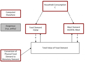
Total food demand in million metric tons consists of the sum of meat demand and food demand. It can be, however, that the monetary value of those calculated demands is greater than the financial ability of households to pay for them. When that is the case, the food and meat demand are proportionately reduced.
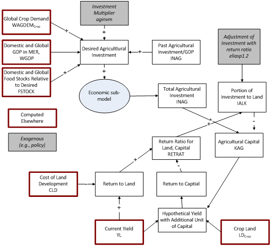
Agricultural Investment and Capital
The level of total desired agricultural investment are driven by the rate of past investment as a
portion of GDP, changes in global crop demand as a portion of GDP, and global crop stocks relative to desired levels. We have experimented also with tying investment to profit rates in agriculture, thereby linking it also to prices relative to costs. The user can use a multiplier to increase or decrease the desired level of investment. This desired amount of investment is passed to the economic model, where it must ‘compete’ with demands for investments in other sectors. The economic model returns a final investment level for use in agriculture.
Investment in agriculture has two possible targets. The first is capital stock. The second is land. The split between the two destinations is a function of the relative returns to cropland development and agricultural capital, the latter of which is determined by the increased yield that could be expected from an additional unit of agricultural capital.
Land Dynamics
In IFs, land use is divided into 5 categories: cropland, grazing land, forest land, "other" land, and urban or built-up land. Four key dynamics are involved in land use change. First, changes in urban land are driven by changes in average income and population, and draws from all other land types. Second, the investment in cropland development is the primary driver of changes in cropland, but this is also influenced by the cost of developing cropland, the depreciation rate, or maintenance cost, of cropland investment, and a user-controllable multiplier. The costs of developing cropland increase as the amount of cropland increases and, therefore, there is less other land available for conversion. Shifts in cropland are compensated by changes in forest and "other" land. Third, changes in grazing land are a function of average income, with shifts again being compensated by changes in forest and "other" land. Finally, conservation policies can influence the amount of forest land, with any necessary adjustments coming from crop and grazing land.
Agricultural Equations
Overview
Briefly, each year the agriculture model begins by estimating the production of crops, meat, and fish. It then turns to the demand for these commodities, followed by trade. The model then looks at changes in stocks and potential shortages related to calorie availability. These influence prices for the coming year, as well as desired investment, which are passed to the economic model, which determines the actual amount of investment that will be available. With this knowledge, the model can then estimate values for changes in land development, agricultural capital, and livestock for the coming year.
This help section presents and discusses the equations that are central to each of these steps in the agricultural model. Along the way, it also presents information related to the actions in the pre-processor and first year of the agriculture model, which are important in setting the stage for the forecasts.
Agricultural Supply
Crop, meat, and fish supply have very different bases and IFs determines them in separate procedures.
Crop Production
Crop production (AGPf=1) i is the product of yield and land devoted to crops (LDl=1).
http://www.du.edu/ifs/help/media/images/ag-module/ageq1.png
We focus here on the determination of yield; the amount of land devoted to crops is addressed in the Land Dynamics section.
Yield functions are almost invariably some kind of saturating exponential that represents decreasing marginal returns on inputs such as fertilizer or farm machinery. Such functions have been used, for instance in World 3 (Meadows, 1974), SARUM, (SARU, 1977), the Bariloche Model (Herrera, et al., 1976), and AGRIMOD (Levis, et al., 1977). IFs also uses a saturating exponential, but relies on a Cobb-Douglas form. The Cobb-Douglas function is used in part to maintain symmetry with the economic model but more fundamentally to introduce labor as a factor of production. Especially in less developed countries (LDCs) where a rural labor surplus exists, there is little question that labor, and especially labor efficiency improvement, can be an important production factor.
In the first year of the model, yield (YL) is computed simply as the ratio of crop production (AGPf=1) to cropland (LDl=1). The determinations of the initial values of these variables are described elsewhere in this document. It is bound, however, to be no greater than 20 tons per hectare in any country.
In forecast years, IFs computes yield in stages. The first provides a basic yield (BYL) representing change in long-term factors such as capital, labor and technology. The second stage uses this basic yield as an input and modifies it based on prices, so as to represent changes in shorter-term factors (e.g. amounts of fertilizer used, even the percentage of land actually under cultivation). Finally, in a third stage, yields are adjusted in response to changing climate conditions.
The basic yield (byl) relates yield to agriculture capital (KAG), agricultural labor (LABS), technological advance (AGTEC), a scaling parameter (CD), an exponent (CDALF), and a saturation coefficient (SATK).
http://www.du.edu/ifs/help/media/images/ag-module/ageq2.png
The equations for KAG and LABS are described elsewhere (see the Capital Dynamics and the economic model, respectively).
cD is a scaling factor calculated in the first year of the model based upon the base year yield (YL), capital (KAG), and labor supply (LABS). It is similar to the shift factors elsewhere in the model, which are used to match predicted values in the base year to actual values. It does not change over time.
http://www.du.edu/ifs/help/media/images/ag-module/ageq3.png
CDALF is the standard Cobb-Douglas alpha reflecting the relative elasticities of yield to capital and labor. It is computed each year in a function, rooted in data on factor shares from the Global Trade and Analysis Project, driven by GDP per capita at PPP.
AGTEC is a factor-neutral technological progress coefficient similar to a multifactor productivity coefficient. It is initially set to 1 and changes each year based upon a technological growth rate (TECHGROAG).
http://www.du.edu/ifs/help/media/images/ag-module/ageq4.png
The algorithmic structure for computing the annual values of TECHGRO involves four elements:
The difference between a targeted yield growth calculated the first year and the portion of that growth not initially related to growth of capital and labor (hence the underlying initial technology element of agricultural production growth); call it AGTECHINIT. This element is assumed to decrease by half over100 years.
The gap between desired global crop stock levels and actual stocks (hence the global pressure for technological advance in agriculture); call it AGTECHPRESS. This contribution is introduced by way of the ADJUSTR function of IFs.[1]
The difference between the productivity of the agricultural sector calculated in the economic model and the initial year's value of that (hence reflecting changes in the contributions of human, social, physical, and knowledge capital to technological advance of the society generally); call if AGMFPLT.
The degree to which crop production is approaching upper limits of potential; this again involves the saturation coefficient (SATK).
The algorithmic structure this is:
http://www.du.edu/ifs/help/media/images/ag-module/ageq5.png
The saturation coefficient is a multiplier of the Cobb-Douglas function and of the technological change element. It is the ratio of the gap between a maximum possible yield (YLLim) and a moving average of yields to the gap between a maximum possible yield and the initial yield, raised to an exogenous yield exponent (ylexp ). With positive parameters the form produces decreasing marginal returns.
http://www.du.edu/ifs/help/media/images/ag-module/ageq6.png
where
sylr is a moving average of byl, the historical component of which is weighted by 1 minus the user-controlled global parameter ylhw .
ylexp global parameter
The maximum possible yield (YLLim) is estimated for each country and can change over time. It is calculated as the maximum of 1.5 times the initial yield (YLr,t=1) and the multiple of an external user-controlled parameter (ylmax ) and an adjustment factor (YLMaxM).
http://www.du.edu/ifs/help/media/images/ag-module/ageq7.png
where
ylmax is a country-specific parameter
The adjustment factor YLMaxM allows for some additional growth in the yields for poorer countries
http://www.du.edu/ifs/help/media/images/ag-module/ageq8.png
where
DevWeightr is the GDPPCPr/30, with a maximum value of 1
YlMaxFound is the maximum value of YL found in the first year
Before moving to the next stage, a check is made to see if the growth in byl is within reason. Specifically, byl is not allowed to exceed the moving average of byl (syl) times a given growth rate (ylgrbound). This bound is the maximum of a user-controlled global parameter - ylmaxgr and an initial country specific target growth rate (tgrylir).[2] This latter target growth rate in yield is set in the first year and is a function of current crop demand (AGDEM), expected crop demand (etdem), and a target growth rate in cropland.
http://www.du.edu/ifs/help/media/images/ag-module/ageq9.png
where
tgrld is a country-specific parameter indicating target growth in crop land
etdem is an initial year estimate of the sum of industrial, feed and food demand for crops in the following year
At this point, the basic yield (BYL) is adjusted by a number of factors. The first of these is a simple country-specific user-controlled multiplier – ylm . ylm can be used to represent the effects of any number of exogenous factors, such as political/social management (e.g., collectivization of agriculture).
The basic yield represents the long-term tendency in yield but agricultural production levels are quite responsive to short-term factors such as fertilizer use levels and intensity of cultivation. Those short-term factors under farmer control (therefore excluding weather) depend in turn on prices, or more specifically on the profit (FPROFITR) that the farmer expects. Because of computational sequence, we use domestic food stocks as a proxy for profit level.
In this second stage, the recomputed yield (YL) is multiplied by a stock adjustment factor.
http://www.du.edu/ifs/help/media/images/ag-module/ageq10.png
The stock adjustment factor uses the ADJSTR function to calculate an adjustment factor related to the current stocks, the recent change in stocks, and a desired stock level. The desired stock level is given as a fraction (agdstl) of the sum of crop demand (AGDEMf=1) and crop production (AGPf=1). agdstl is set to be 1.5 times dstl , which is a global parameter that can be adjusted by the user.
The focus in IFs on yield response to prices differs somewhat from the normal use of price elasticities of supply. For reference, Rosegrant, Agcaoili-Sombila, and Perez (1995: 5) report that price elasticities for crops are quite small, in the range of .05 to .4.
In the third stage. IFs considers the potential effects of a changing climate on crop yields. This is separated into two parts: the direct effect of atmospheric carbon dioxide concentrations and the effects of changes in temperature and precipitation.
The direct effect of atmospheric carbon dioxide assumes a linear relationship between changes in the atmospheric concentration from a base year of 1990 and the percentage change in crop yields.
http://www.du.edu/ifs/help/media/images/ag-module/ageq11.png
where
envco2fert is a global, user-controllable parameter
CO2PPMt=1990 is hard coded as 354.19 parts per million
The effect of changes in annual average temperature and precipitation are based upon two assumptions: 1) there is an optimal temperature (Topt) for crop growth, with yields falling both below and above this temperature and 2) there is a logarithmic relationship between precipitation and crop yields. The choice of this functional form was informed by work reviewed in Cline (2007). Together, these result in the following equation:
http://www.du.edu/ifs/help/media/images/ag-module/ageq12.png
where
T0 and P0 are country-specific annual average temperature (degrees C) and precipitation (mm/year) for the period 1980-99.
DeltaT and DeltaP are country specific changes in annual average temperature (degrees C) and precipitation (percent) compared to the period 1980-99. These are tied to global average temperature changes and described in the documentation of the IFs environment model.
Topt is the average annual temperature at which yield is maximized. It is hard coded with a value of 0.602 degrees C.
SigmaTsqd is a shape parameter determining how quickly yields decline when the temperature moves away from the optimum. It is hard coded with a value of 309.809.
CO2Fert and ClimateEffect are multiplied by each other to determine the effect on crop yields.
There are two final checks on crop yields. They are not allowed to be less than one-fifth of the estimate of basic yield (BYL) and they cannot exceed the country-specific maximum (ylmax ) or 50 tons per hectare.
[file:///C:/Users/Ara/Desktop/Agricultural%20Documentation%20v19_AG.docx#_ftnref1 [1]] The ADJSTR function, used throughout the model, is a PID controller that builds in some anticipatory and smoothing behavior to equilibrium processes by calculating an adjustment factor. It considers both the gap between the current value of the specific variable of interest, here crop stocks, and a target value, as well as change in the gap since the last time step. Two parameters control the degree to which these two "differences" affect the calculation of the adjustment factor. In this case, these are the global, user-controllable parameters elfdpr1 and elfdpr2 .
[file:///C:/Users/Ara/Desktop/Agricultural%20Documentation%20v19_AG.docx#_ftnref1 [2]] There is also an adjustment whereby ylmaxgr is reduced for countries with syl>5, falling to a value of 0.01 when syl>=8.
Meat Production
Meat production, in metric tons, is given as the multiple of the herd size (LVHERD) and the slaughter rate (slr ). The latter is a global parameter.
http://www.du.edu/ifs/help/media/images/ag-module/ageq13.png
The dynamics of the livestock herd are described in the Livestock Dynamics section.
Fish Production
The production of fish has two components, wild catch and aquaculture. Total global wild fish catch (ofscth ), and each region's share in it (rfsshr ) are exogenous parameters that can be set by the user.
The amount of aquaculture (AQUACUL) in the first year is provided by historical data; these values can be modified by the user. Production is assumed to grow over time. The default growth rate in the first year for all countries is 3.5 percent, but this value can be modified by the user, by country, with the parameter aquaculgr . This growth rate declines to 0 over a number of years given by the global parameter aquaculconv . Finally, users can change the amount of aquaculture production, by country, with the multiplier aquaculm .
http://www.du.edu/ifs/help/media/images/ag-module/ageq14.png
where
aquaculgrr,t declines from aquaculgrr,t=1 to 0 over aquaculconv years
Total fish production (FISH) is given as:
http://www.du.edu/ifs/help/media/images/ag-module/ageq15.png
Production Losses
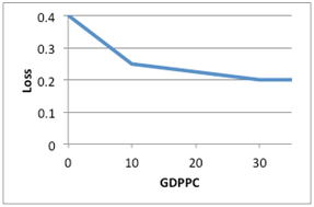
Some food production will never make it to markets, but will be lost in the field or in distribution systems to pests, spoilage, etc. For crops, an initial estimate of the loss in the first year, LOSSI, is given as a function of GDP per capita using a table function that captures the tendency of loss to decrease with higher income levels (see figure below). This is reset to 0 in the pre-processor if the estimate of cereal production in the first year is zero. If the loss seems too high, specifically if it is greater than or equal to 0.9 - cereal exports/cereal production, then the loss for crops is recomputed as the maximum of 0.05 and 0.9 – cereal exports/cereal production. The estimate of loss in the first year for meatis assumed to be one-half of the initial estimate for crops; no losses are assumed for fish. In future years, for crops and meat, the loss is calculated as the loss in the first year multiplied by the ratio of the loss estimated from the table function above using current GDP per capita to GDP per capita in the first year; therefore, as GDP per capita increases relative to the first year, loss decreases. A common loss multiplier (lossm ) is also available, allowing users to adjust crop and meat losses. Finally, losses are bound between 0 and 0.8. At present, fish loss remains constant at 0 for all years.http://www.du.edu/ifs/help/media/images/ag-module/ageq16.png
Agricultural Demand
IFs computes demand for three agricultural categories—crops, meat, and fish. Total human food demand (for both crops and meat) is responsive to calorie demand, which in turn responds to GDP per capita (as a proxy for income). The division of calorie demand between demand for calories from crops and from meat changes in response also to GDP per capita (increasing in income). The calculation sequence of human food demand in IFs thus begins with determination of calorie demand, determines how much of that is satisfied by the typically increasing share from meat (bounding that share with reasonable upper limits), and how much remains to be satisfied from crops. At this point IFs does not track calories from fish. Once the remaining needed calories from crops are determined, the physical demand for crops in million metric tons can also be determined.
Crop demand also involves demand for industrial use and animal feed. Total crop demand is the sum of those two demands and that for food crops.
Initial Agricultural Demands
A common process across categories is used to estimate initial values for the first years. It relies upon the first year values of production, imports, exports, and losses, all of which are generated in the pre-processor and discussed elsewhere in this document, to compute an apparent level of demand or consumption. The reason for this is that demand data are much less available for food and agriculture than are production and trade data. An initial estimate of demand in each category is given as the sum of post-loss production and imports minus exports:
http://www.du.edu/ifs/help/media/images/ag-module/ageq17.png
An initial portion of this first estimate of demand is set aside for the purposes of satisfying the need for growth in food stocks as underlying total food demand and supply change (using initial economic growth as a proxy for that annual stock growth). See also the section on stocks. That adjusted demand then becomes the basis, along with production, for an estimate of food stocks.
http://www.du.edu/ifs/help/media/images/ag-module/ageq18.png
where
agdstl is a parameter used to set desired stock levels for agricultural commodities. It is set to be 1.5 times dstl , which is a global parameter that can be adjusted by the user
igdpr is the initial growth rate in GDP
Given the resulting initial model year value for food stocks, it is then possible to calculate a more precise increment of stock change needed and add that back into the demand.
http://www.du.edu/ifs/help/media/images/ag-module/ageq19.png
In the first year of the model, a predicted level of calories per capita (CalPerCap) is estimated as an increasing function of average income.[1] This is bound from above by an assumed maximum value, given by the global parameter calmax .
The predicted per capita value is converted to total calorie demand (caldem) by multiplying by the population (POP). A multiplicative shift factor (calactpredrat), used in the forecast years, is then calculated by dividing by the value of calories available (CLAVAL) by this demand.
http://www.du.edu/ifs/help/media/images/ag-module/ageq20.png
where
CLAVAL is calorie availability; its calculation is described below in the section on calorie availability
This value of calactpredrat gradually converges to 1 over a period given by the global parameter agconv and appears in future equations with the name adjustforinitialdevc.
In the forecast years, a predicted value of per capita calorie demand (CalPerCap) is once again calculated as a function of average income using the equation above, with a maximum value given by calmax . A base level of calories per capita (calbase) is also calculated, which is given as the minimum of 3000 or calmax minus 300. Because comparative cross sections show a growth of around 4 calories per capita per year independent of average income, a factor representing this increase (caldgr) is calculated as:
http://www.du.edu/ifs/help/media/images/ag-module/ageq21.png
Thus, depending on the exact values of calmax , calbase, and CalPerCap, caldgr grows each year by a value that centers around 4 calories. This value is then added to the predicted value in calculating the total demand for calories. The equation also takes into account calmax and the multiplicative shift factor on calories per capita noted above.
http://www.du.edu/ifs/help/media/images/ag-module/ageq22.png
This total calorie demand is divided into demand from meat and demand from crops. Meat demand in tons (AGDEM, category 2) is discussed in the following section. Here we focus on how this is converted to calories. Two country-specific parameters, lvcfr and sclavf, calculated in the first year of the model are key to this conversion.
lvcfr is a country-specific factor converting livestock in tons to calories. This is initially set equal to the global parameter lvcf , but may be adjusted downward. This is done in cases where the initial estimate of the share of calories from meat exceeds a maximum value: given by t, i.e., if
http://www.du.edu/ifs/help/media/images/ag-module/ageq23.png
where
calmeatm is a global parameter indicating the maximum share of calories to come from meat
In this case, lvcfr is repeated reduced by 10 percent until the share of total calories coming from meat falls below calmeatm .
sclavf is a country-specific multiplicative shift factor that converts the total annual demand for food crops and crop equivalents from meat to daily calorie availability
http://www.du.edu/ifs/help/media/images/ag-module/ageq24.png
Note that sclavf can take on a value greater that or less than 1.
lvcfr and sclavf maintain the same value in all the forecast years.
[file:///C:/Users/Ara/Desktop/Agricultural%20Documentation%20v19_AG.docx#_ftnref1 [1]] Equation is CalPerCap = 2180.6+368.87*ln(GDPPCP).
Meat Demand and Its Calorie Contribution
In the first model year apparent meat demand is used to compute the calories that its consumption contributes to the need of the population. In subsequent years the calculations begin with meat demand again, and conclude with calculation of the calories provided by it. This is needed subsequently to determine the calories required from crops.
In the first year of the model's forecasts an apparent consumption of meat is calculated as for other agricultural demand components (in terms of production plus imports and subtracting exports). In the first year, two other country-specific values are calculated that are used to estimate this value in the forecast years—meatmaxr and meatactpredrat.
meatmaxr is a country-specific maximum for per capita meat demand in tons. It is calculated as the maximum of a global parameter (meatmax ) and per capita total meat demand (AGDEM, category 2 divided by POP).
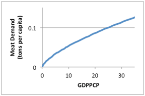
meatactpredrat, which acts as a shift factor, is the ratio of actual total meat demand (in tons) to a predicted value (MeatDem). First, a predicted per capita value is estimated as an increasing function of GDP per capita[1] :This is not allowed to exceed meatmaxr and is then multiplied by the population to yield the predicted value of total MeatDem. meatactpredrat is then calculated as
http://www.du.edu/ifs/help/media/images/ag-module/ageq25.png
meatmaxr is held constant in all forecast years. For most countries, the value of meatactpredrat gradually converges to 1 over a period given by the global parameter agconv . The exception is for certain countries in South Asia, specifically India, Nepal, and Mauritius, for which it does not converge. In either case, it is represented in equations in future year as adjustforinitialdevm.
In the forecast years, IFs then computes the demand for meat in tons as a function of population, average income, world food prices, the shift factor, and a multiplier that allows users to directly increase or decrease demand. As in the first year, per capita demand (tonspercap) is initially estimated as a function of average income, using the same function presented above. This is then converted to total demand in the following equation.
http://www.du.edu/ifs/help/media/images/ag-module/ageq26.png
where
elasmd is a global parameter representing the elasticity of meat demand to changes in the world price relative the first year
A number of further adjustments are made to the meat demand, in the following order:
- The estimated value is restricted to be no greater than that given by multiplying the size of the population (POP) by the maximum for per capita meat demand in tons (meatmaxr)
- This adjusted value is multiplied by a demand multiplier (agdemmr,f=2 ), which can raise or lower demand.
- If the initial estimate of calories from meat (calfrommeat) exceeds the maximum amount of calories allowed to come from meat, given by calmeatm * caldem, then the demand for meat in tons is recalculated as:
http://www.du.edu/ifs/help/media/images/ag-module/ageq27.png
Note that this implies a reduction in the total demand for meat in tons.
In order to undertake the third adjustment, and to prepare for the calculation of calories needed from crops, the meat demand needs to be converted from tons to calories. An initial estimate of calories from meat (calfrommeat) is calculated from the total demand for meat in tons, adjusted by lvcfr and sclavf:
http://www.du.edu/ifs/help/media/images/ag-module/ageq28.png
Should this exceed the maximum amount of calories allowed to come from meat, given by calmeatm * caldem, then two adjustments are made. First, calfrommeat is set equal to this maximum amount
http://www.du.edu/ifs/help/media/images/ag-module/ageq29.png
and the total demand for meat in tons is recalculated
http://www.du.edu/ifs/help/media/images/ag-module/ageq30.png
Note that this implies a reduction in the total demand for meat in tons.
Now that the demands for total calories and calories from meat are known, calories to be demanded from crops (mostly grain) can be calculated simply as
http://www.du.edu/ifs/help/media/images/ag-module/ageq31.png
[file:///C:/Users/Ara/Desktop/Agricultural%20Documentation%20v19_AG.docx#_ftnref1 [1]] Equation is Meat Demand per Capita = .0109999999403954GDPPCP0.684800028800964.
Fish Demand
Currently IFs does not calculate calories from fish and determine that contribution to total calorie demand. We anticipate that model extension in the future.
The calculation of fish demand (AGDEM, category 3) in the first year was described at the start of the Demand section as having the same apparent consumption approach as used for other agricultural demands (production plus imports minus exports and adjustment stocks). In the first year, a calculation is also made of fish demand per capita (fishdemipc), which is simply the ratio of AGDEM, category 3 to population (POP).
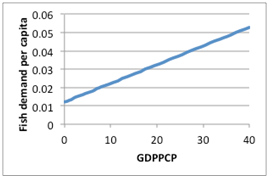
In the forecast year, fish demand per capita is assumed to grow with growth in average income, with some adjustments. First, predicted values for fish demand per capita are calculated as a function of income in the first and current year using the function depicted in the diagram below[1] .
The initial estimate of fish demand per capita is the value for the initial year (fishdemipc) multiplied by the ratio of the predicted value in the current year (tonspercap) to the predicted value in the first year (tonspercapi)
http://www.du.edu/ifs/help/media/images/ag-module/ageq32.png
Once the per capita demand exceeds 50 percent of the initial value, a new logic kicks in.
fishdempc is also not allowed to exceed the value in the first year or 0.1, whichever is larger.
Finally, total demand for fish is determined by multiplying the per capita value by the population (POP), with a price adjustment.
http://www.du.edu/ifs/help/media/images/ag-module/ageq33.png
[file:///C:/Users/Ara/Desktop/Agricultural%20Documentation%20v19_AG.docx#_ftnref1 [1]] Equation is Fish Demand per Capita = 0.0121 + 0.00102*GDPPCP
Crop Demand for Food (FDEM) and Its Calorie Contribution
Total crop demand (AGDEM, category 1) has three components: feed (FEDDEM), industrial (INDEM) and food (FDEM). Here we describe the basic calculations for food use of crops. Note that in forecast years additional adjustments are made to a number of the demand variables, so the discussion here will not fully complete the determination of FDEM.
The demand for crops for food in the base year is not computed in the pre-processor. Rather, in the first year of the model, the demand for crops for food (FDEM) is calculated as the residual of total agricultural demand for crops minus the demand for crops for feed and for industry.[1]
http://www.du.edu/ifs/help/media/images/ag-module/ageq34.png
Given earlier calculations of the total demand for calories and of the share of that demand to be met by meat, it was possible to calculate the calories needed from crops, mostly grain around the world (calfromgrain). From this it is possible to calculate food demand using the factor relating the conversion from crops to calories (sclavf), an adjustment based on world crop prices, and a multiplier that can be used to increase or decrease demand.
http://www.du.edu/ifs/help/media/images/ag-module/ageq35.png
FDEM is bound from above based on the assumed maximum calories per capita (calmax ), and the multiplicative shift factor on calories per capita (adjustforinitialdevc).
http://www.du.edu/ifs/help/media/images/ag-module/ageq36.png
[file:///C:/Users/Ara/Desktop/Agricultural%20Documentation%20v19_AG.docx#_ftnref1 [1]] It is bound to be between 0.1 and 1000.
Feed Demand for Crops
Feed demand represents the amount of crops that need to be produced to complement what livestock receive from grazing.
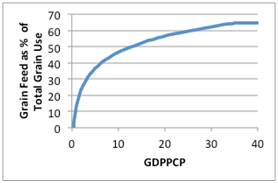
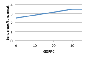
In the pre-processor, feed demand (FeedDem) is initially estimated as a percentage of the apparent consumption of cereals, which grows with average income, implying that as countries develop, more of their grain production is used to feed livestock. The function is depicted on the right[1] :If the model estimates that the productivity of grazing land in terms of feed equivalent produced per unit area is below a minimum level, however, then FeedDem is adjusted downward. It determines this by first estimating the feed requirements per unit livestock (fedreq). This is estimated as an increasing function of average income as shown in the figure below.
This function takes into account the fact that at low levels of income most meat consumption is typically poultry (with a conversion ratio of grain to meat of about 2-to-1), while at higher levels of income, pork (4-to-1) and then beef (7-to-1) become increasing portions of meat demand (Brown, 1995: 45-47).
With the value of fedreq, the productivity of grazing land can be estimated as the difference between the total feed requirement for the number of livestock minus the feed demand divided by the amount of grazing land.
http://www.du.edu/ifs/help/media/images/ag-module/ageq37.png
where
LiveHerd is the size of the livestock herd
LDGraz is the amount of grazing land
If the value of GLandCAP is less than a minimum (MinLDProd—currently hard coded as 0.01 tons of meat per hectare, based on values for the Saudi desert), then FeedDem is recalculated as the difference between the total feed requirement for the number of livestock minus the amount of feed equivalent produced by grazing using the minimum productivity.
http://www.du.edu/ifs/help/media/images/ag-module/ageq38.png
Note that this occurs when the feed from crops meets most, if not all, of the total feed requirements, implying little or no need for feed equivalents from grazing land.
In the first year of the model, grazing land productivity (now called GLDCAP) and an adjustment to feed requirements per unit livestock (fedreqm) are calculated for each country. GLDCAP is initially back-calculated based on the known values of the size of the livestock herd (now called LVHERD), the feed requirement per unit livestock (fedreq —calculated as a function of GDPPC as shown above), the feed demand (now called FEDDEM), and the amount of grazing land (now called LDl=2):
http://www.du.edu/ifs/help/media/images/ag-module/ageq39.png
This yields a productivity of grazing land that perfectly meets the difference between the total feed requirement and that provided by crops.
Again, if the calculated value of GLDCAP is less than the assumed minimum level (MinLDProd), however, then adjustments are made. First, an adjustment factor (fedreqm) is calculated by assuming that a minimum amount of feed equivalents from grazing land are produced even if this results in a total amount of feed that is larger than necessary to meet the total feed requirement:
http://www.du.edu/ifs/help/media/images/ag-module/ageq40.png
Note that this value is always greater than or equal to 1 given the condition for making the adjustment. When no adjustment is made, fedreqm is set to 1.
After the calculation of this adjustment factor, GLDCAP is recalculated as
http://www.du.edu/ifs/help/media/images/ag-module/ageq41.png
which basically implies that GLDCAP will always at least as large as MinLDProd after the adjustment.
The values of GLDCAP and fedreqm calculated in the first year are held constant for all forecast years
In the forecast years, FEDDEM is calculated as a function of the size of the livestock herd (LVHERD), the feed requirements per unit livestock (fedreq), the amount of grazing land (LDl=2), and the productivity of grazing land (GLDCAP), but adjustments are also made reflecting the effect of global crop prices on grazing intensity (WAPf=1), changes in the efficiency with which feed is converted into. meat, and the adjustment factor fedreqm calculated in the first year. There is also a parameter with which the user can cause a brute force increase or decrease in FEDDEM (agdemmf=1 ).
The model first calculates the amount of crop equivalent produced from grazing land using the following equation:
http://www.du.edu/ifs/help/media/images/ag-module/ageq42.png
where
elglinpr is a global parameter for the elasticity of livestock grazing intensity to annual changes in world crop prices; the basic assumption is that increasing prices should lead to increased grazing intensity and therefore greater productivity of grazing land[2] .
This production of crop equivalents from grazing land is then subtracted from total feed requirement in the following equation:
http://www.du.edu/ifs/help/media/images/ag-module/ageq43.png
where
livhdpro is a global parameter related to the rate at which the productivity of crops in producing meat improves over time. This part of the equation implies that the amount of feed needed to produce a unit of meat declines over time to a minimum of half the original amount required
agdemm (category 1) is a country-specific multiplier that can be used to increase or decrease crop demand
[file:///C:/Users/Ara/Desktop/Agricultural%20Documentation%20v19_AG.docx#_ftnref1 [1]] The specific equation is 13.427 +14.421*ln(GDPPCP), up to GDPPCP=35. The code sets minimum and maximum values of 1 and 80 percent, respectively.
[file:///C:/Users/Ara/Desktop/Agricultural%20Documentation%20v19_AG.docx#_ftnref1 [2]] The code, as written, ignores price effects that would reduce GLFeedEq. Since elglinpr is generally positive, this implies that decreases in world crop prices are ignored.
Industrial Demand for Crops
Industrial demand for crops (IndDem) is initially estimated for the first year in the pre-processor. It is determined, arbitrarily, as one tenth of crop supply, which equals post loss crop production plus imports minus exports.
http://www.du.edu/ifs/help/media/images/ag-module/ageq44.png
It can then be decreased (increased) if the initial estimates of crop demand for food are considered too low (high).
In the first year, two values related to industrial demand for crops (now called INDEM) are calculated. The first of these is a multiplicative shift factor (INDEMK), which is calculated as the ratio of relates actual to predicted industrial demand for crops. The predicted value is given by a function that relates per capita industrial demand to GDP per capita, which is shown below.[1] This multiplicative shift factor remains constant over time.The same function is used to calculate an expected demand for the next year (eindem). The predicted value from the function is computed using the expected level of GDP per capita (egdppcp); this value is multiplied by the expected population (epop) and the multiplicative shift factor (INDEMK) to calculate the expected demand. This expected demand is used in conjunction with the expected demands for crops for feed and crops for food to determine the initial target growth rate in yield (tgryli) discussed in the section on crop production above.
In the forecast years, the initial value of industrial demand for crops is also estimated using the table function above to get a predicted value for industrial demand per capita, which is then multiplied by population (POP) and the multiplicative shift factor (INDEMK). At this point, a region-specific multiplier (agdemmf=1 ) can either increase or decrease the initial estimate of INDEM.
The first adjustment to INDEM is related to the world energy price (WEP) and reflects the use of crops for fuel production. Specifically, as the world energy price increases relative to the price in the first year, the industrial demand for crops increases.
http://www.du.edu/ifs/help/media/images/ag-module/ageq45.png
where
WEP is world energy price
FoodforFuel is the elasticity of industrial use of crops to world energy prices. It starts at a value given by the global parameter elagind , and declines to a value of 0 over 50 years.
The second adjustment relates to the world crop price (WAPf=1); as this increases relative to the price in the first year, industrial demand for crops declines.
http://www.du.edu/ifs/help/media/images/ag-module/ageq46.png
where
WAP is world crop price
elascd is a global parameter specifying the elasticity of crop demand to global food prices
A third adjustment is based on an assumed cap on per capita industrial demand for crops (IndemCapperPop —hard coded, declines from 0.17 to 0.12 over 50 years). Specifically, INDEM is not allowed to exceed IndemCapperPop * POP.
Finally, INDEM can be reduced if the sum of expenditures on food crops at world prices (FDEM*WAPf=1) and meat (AGDEMf=2*WAPf=2) exceeds 85 percent of household consumption expenditures as calculated in the economic model.
[file:///C:/Users/Ara/Desktop/Agricultural%20Documentation%20v19_AG.docx#_ftnref1 [1]] Equation is INDEM = 0.0376 + 0.000704 * GDPPCP
Final Agricultural Demand Adjustments in Forecast Years
Two final adjustments are made to a number of the agricultural demand variables in the forecast years. First, if the total per capita calories from meat and crops exceed the maximum calories, i.e.
http://www.du.edu/ifs/help/media/images/ag-module/ageq47.png
then the demand for crops for food and the demand for meat in tons are scaled by the ratio of the maximum to the estimated calories
http://www.du.edu/ifs/help/media/images/ag-module/ageq48.png
Second, if the preliminary estimate of total food demand in monetary terms (csprelim), is too large of a share of consumption, i.e., if
http://www.du.edu/ifs/help/media/images/ag-module/ageq49.png
where
CSF is the ratio of consumer spending in the agricultural sector in the first year (CSr,s=1,t=1) to DemValr, a weighted sum of demands for agricultural products for food in the first year
http://www.du.edu/ifs/help/media/images/ag-module/ageq50.png
C is total household consumption in the first year
When this is the case, a series of steps are taken to bring these values back in line.
1. The necessary reduction (necreducr), which is in monetary terms, is calculated as csprelimr – 0.85*Cr
2. A reduction factor (reducfact) is calculated as
http://www.du.edu/ifs/help/media/images/ag-module/ageq51.png
with a maximum value of 1
3. The physical demands for crops for feed (FEDDEM), crops for industry (INDEM), and meat in tons (AGP, category 2) are all reduced by reducfact, and the value of the meat reduction is saved for the next step
http://www.du.edu/ifs/help/media/images/ag-module/ageq52.png
4. An estimate of the necessary reductions in crops for food, in monetary terms is estimated by subtracting the savings obtained through the reduction in meat demand
http://www.du.edu/ifs/help/media/images/ag-module/ageq53.png
5. The physical demand for crops for food (FDEM) is then reduced as follows
http://www.du.edu/ifs/help/media/images/ag-module/ageq54.png
Note that this ensures that FDEM is not reduced by more than ninety percent.
Finally, given the changes above, the total demand for crops is recalculated as the sum of the final values of feed, industry, and food demand.
http://www.du.edu/ifs/help/media/images/ag-module/ageq55.png
Trade
Consistent with the approaches within both the economic model and the energy model, trade of agricultural products in IFs uses a pooled approach rather than a bilateral one. That is, we can see the total exports and imports of each country/region, but not the specific volume of trade between any two. Offered exports and demanded imports from each country/region are responsive to the past shares of export and import bases and are summed globally. The average of the totals is taken as the actual level of global trade and the country exports and imports are normalized to that level.
Price differentials across countries do not influence agricultural trade. Although the IFs project has experimented over time with making such trade responsive to prices, there is an increasing tendency globally for food prices to be more closely aligned across countries than was true historically. Moreover, the use within IFs of local relative food surpluses or deficits (as indicated by stock levels) to adjust trade patterns is an effective proxy for the use of prices.
The initial year values of the imports (AGM) and exports (AGX) of the three agricultural commodities in physical quantities are determined in the pre-processor. Since we only have historical data on the imports and exports of fish in monetary terms, these need to be converted to physical terms. This is done by multiplying the monetary values, which are in $billion, by 1000*/2200 to get physical values in million tons. In addition, exports of fish are limited to be less than 70 percent of total fish available and imports less than 1 percent of total fish available. For each of the three agricultural commodity groupings, if there is an imbalance between global imports and global exports in the preprocessor, the latter takes precedence and national imports are adjusted to bring global imports into line with global exports.
In the first year, seven variables are set related to trade for each commodity: XKAVE, MKAVE, XKAVMAX, MKAVMAX at the country level and wxct=1, wmdt=1, and WAPt=1 at the global level.
XKAVE and MKAVE are moving average values of export and import propensity, respectively. They are specified as the ratio of agricultural exports and imports to a base value (xbase) for each commodity. For exports, this is basically the sum of production and demand for that commodity; for imports, it is just demand.
http://www.du.edu/ifs/help/media/images/ag-module/ageq56.png
XKAVMAX and MKAVMAX are maximum values of XKAVE and MKAVE. For crops and meat, XKAVMAX is set to 1.1 times XKAVE, but is not allowed to exceed a value of 0.7; MKAVMAX is set to 1.5 times XKAVE, but also is not allowed to exceed a value of 0.7. For fish, XKAVMAX is set to 1.1 times XKAVE, with a bound of 0.95; MKAVE is set to 1.5 times MKAVE, with a bound of 2. These values are held constant for all future years.
XPriceTermLag, and MPriceTermLag are set to 0 for all commodities. wxc and wmd are the total world agricultural exports and imports; these are set to a value of 1 in the first year. WAP is the initial world price index for each commodity, which is set to 100.
In the forecast years, the process for determining agricultural imports and exports involves the following steps:
- Estimating the agricultural export capacity and agricultural import demand for each country.
- Reconciling the differences between global agricultural export capacity and global agricultural import demand.
- Computing the actual levels of agricultural exports and agricultural imports for each country
The agricultural export capacity is estimated by multiplying the export propensity (XKAVE) by the current year’s production and demand. It is also limited by XKAVMAX:
http://www.du.edu/ifs/help/media/images/ag-module/ageq57.png
Similarly, the agricultural import demand is estimated by multiplying the import propensity (MKAVE) by the current year’s demand, with a limit set by MKAVMAX
http://www.du.edu/ifs/help/media/images/ag-module/ageq58.png
For each country, values are also estimated for its net surplus or deficit (surpdef) for each commodity. This is based on the following factors: 1) post-loss production, 2) domestic demand, 3) the difference between current and desired stocks, and 4) a trade term
http://www.du.edu/ifs/help/media/images/ag-module/ageq59.png
The first three factors are straightforward. Production minus demand reflects a basic net surplus, which is then adjusted by any net surplus in stocks. The TradeTerm is related the relative role a country plays in global imports and exports and is given as:
http://www.du.edu/ifs/help/media/images/ag-module/ageq60.png
The TradeTerm is positive (negative) when a country has a larger (smaller) share of the global imports than it does of the global exports of a particular commodity and vice versa. Since the TradeTerm is is added to surpdef, it acts as a balancing mechanism; countries that appear as relatively larger (smaller) importers get a positive (negative) boost to their estimated net surplus, which tends to reduce (increase) imports as shown below.
At this point, the global sum of exports and imports across countries will likely differ. Therefore, a procedure is required to balance these. In preparation for this one more global variable and several country-level variables are calculated. The global variable is globalsurdefrate, which is the ratio of the sum across countries of net surplus divided by the sum across countries of demand and production, which is the stock base.
http://www.du.edu/ifs/help/media/images/ag-module/ageq61.png
The country-level variables are as follows:
The first term modifies the country’s net surplus, increasing (decreasing) it when the global net surplus is negative (positive).
http://www.du.edu/ifs/help/media/images/ag-module/ageq62.png
The second term modifies how rapidly the net surplus is closed.
http://www.du.edu/ifs/help/media/images/ag-module/ageq63.png
The third term is simply the ratio of exports to the sum of imports and exports.
http://www.du.edu/ifs/help/media/images/ag-module/ageq64.png
The next step is to calculate whether it is necessary to increase (decrease) imports and decrease (increase) exports for each country, and by how much. Whether a country needs to increase its initial estimates of imports and decrease its initial estimates of exports, or vice versa, is determined by the sign of countryextrasurdef. If this value is negative, i.e., the country has a net deficit, it will need to reduce exports and increase imports. The opposite holds for when countryextrasurdef is positive.
As for the amount by which imports and exports need to be increased or decreased, this is a function, in general, of the size of the necessary adjustment and the export share:
http://www.du.edu/ifs/help/media/images/ag-module/ageq65.png
Note that the sign of countryextrasurdef and the fact that exportshare is a value between 0 and 1 ensure that when exports increases, imports fall, and vice versa.[1] Finally, in this adjustment process, exports and imports are not allowed to fall by more than half or more than double.
This process may not fully reconcile global trade, so a final adjustment is made by setting world trade (WT) as the average of global exports and imports and then adjusting the country values accordingly:
http://www.du.edu/ifs/help/media/images/ag-module/ageq66.png
IFs can now update the moving average export (XKAVE) and import (MKAVE) propensities for the next time step. The weights given to history are set by the global parameters xhw and mhw . For small exporters, i.e., where exports are less than one tenth of the sum of production and demand, xhw is reduced by 40 percent, allowing for faster adjustment. XKAVE and MKAVE are updated as
http://www.du.edu/ifs/help/media/images/ag-module/ageq67.png
For crops, the import propensity is bound from below by a factor given by potential GDP (GDPPOT), demand (AGDEM), the conversion factor between agricultural imports in physical terms and dollar values (msf, see section on links to the economic model), and the initial world price for agriculture (WAP).
http://www.du.edu/ifs/help/media/images/ag-module/ageq68.png
Finally, XKAVE and MKAVE are bound from above by XKAVMAX and MKAVMAX, respectively.
[file:///C:/Users/Ara/Desktop/Agricultural%20Documentation%20v19_AG.docx#_ftnref1 [1]] Two other variables, defadjmul and ImportBoost, are included in the calculations to make some finer adjustments to the changes in exports and imports; these relate to the observed behavior for specific countries and are not discussed in detail here. <header><hgroup>
Stocks
</hgroup></header> Due to a lack of good historical data, in the first year, stocks for all three agricultural commodities are assumed to equal desired stocks. These are set to a fraction (agdstl) of total production (AGP) and demand (AGDEM) for each commodity.
http://www.du.edu/ifs/help/media/images/ag-module/ageq69.png
where
agdstl is a parameter used to set desired stock levels for agricultural commodities. It is set to be 1.5 times dstl , which is a global parameter that can be adjusted by the user
In future years, basic stock levels (cumstk) increase with production (AGP) as adjusted for loss before reaching market (LOSS), decrease with demand or consumption (AGDEM), and adjust for net imports (AGM-AGX).
http://www.du.edu/ifs/help/media/images/ag-module/ageq70.png
Of course, the actual stock values (FSTOCK) are not allowed to go negative. If the basic stock level is negative, stocks are set at zero and a shortage (SHO) exists, which affects calorie availability. If the basic stock level is positive there is no shortage and stocks equal the basic level.
http://www.du.edu/ifs/help/media/images/ag-module/ageq71.png
Calorie Availability
Daily per capita calorie availability (CLPC) is initialized in the pre-processor. Where available, data is taken from the FAO[1] . It is multiplied by population (POP) to yield total daily calorie availability and brought into the model with the name CLAVAL. We already saw that this first year value is used in the calculation of two country-specific factors: 1) calactpredrat, which is a shift factor determined as the ratio of calorie availability to predicted calorie demand in the first year, and 2) sclavf, which is a conversion factor relating the total annual demand for food crops and crop equivalents from meat to daily calorie availability.
In the forecast years, CLAVAL depends upon the demand for food crops and meat, but also any shortages in crops or meat. The specific shortage is calculated as
http://www.du.edu/ifs/help/media/images/ag-module/ageq72.png
CLAVAL is then calculated as
http://www.du.edu/ifs/help/media/images/ag-module/ageq73.png
Calorie availability combines with regional calorie need in the population model for the calculation of possible starvation deaths (a seldom used variable because in official death statistics people do not die of starvation but rather of diseases associated with undernutrition); the population and health models therefore look instead to the impact of calorie availability on undernutrition and health.
[file:///C:/Users/Ara/Desktop/Agricultural%20Documentation%20v19_AG.docx#_ftnref1 [1]] Note this occurs in DATAPOP, not DATAAGRI. The historic data series is SERIESCalPCap. Missing data are estimated based on access to water and sanitation or average income.
Prices
IFs keeps track of both national (FPRI) and world (WAP) price indices for each of the three agricultural commodities. All of these are set to an index value of 100 in the building of the base.
The national crop price indices (FPRI, category (1) respond to: 1) changes in global costs of crop production, the latter being expressed as the ratio of global accumulated capital investment in crops to global production and 2) changes in the level of domestic crop stocks. The first factor should provide a long-term basis for rising or falling prices tied to changing technology and other factors of production; the second factor generally should represent shorter-term market variations from that long-term level.
The impact of global costs is given by dividing the ratio of global investment in crops to global production (wkagagpr) in the current year to that same ratio in the first year. The effect of stocks on crop prices (Mul) is calculated using the same ADJSTR function introduced in the description of crop supply, which considers the difference between both the current crop stocks and a desired vale and between current crop stocks and those in the previous year. Two parameters control the degree to which these two ‘differences’ affect the calculation of the adjustment factor. In this case, these are the global, user-controllable parameters fpricr1 and fpricr2 . All together the equation for domestic crop price indices in the coming year is given as
http://www.du.edu/ifs/help/media/images/ag-module/ageq74.png
The domestic crop price indices are also bound between 0.01 and 1000.
The national meat price indices are linked the global crop price. Specifically, they are given as a moving average of the global crop price index.
http://www.du.edu/ifs/help/media/images/ag-module/ageq75.png
where
fprihw is a global parameter used to control the speed at which the domestic meat price changes.
The national fish price indices are all set equal to the global fish price index. The determination of the global fish price is similar to that for the national crop price, but here the stock of interest is the global stock and there is no effect related to costs. The ADJSTR function is used once again to calculate the adjustment factor (MUL), this time focusing on the desired global fish stock, the difference between this and the current global fish stock, and the change in the global fish stock in the past year. Again, two parameters control the degree to which these two "differences" affect the calculation of the adjustment factor. In this case, these are the global, user-controllable parameters fprim1 and fprim2 [file:///C:/Users/Ara/Desktop/Agricultural%20Documentation%20v19_AG.docx#_msocom_1 [U1]] . The global and national fish prices are thus calculated as
http://www.du.edu/ifs/help/media/images/ag-module/ageq76.png
The world price indices for crops and meat are computed, in the following year, as a weighted average of the domestic prices, with the weights given by crop and meat production:
http://www.du.edu/ifs/help/media/images/ag-module/ageq77.png
Returns and Profits
IFs estimates the net returns in agriculture (AGReturn) for each commodity, based upon production costs and net revenues. Agricultural profits (FPROFIT) depend on the gross returns to production (GReturn) relative to the costs of production. At some points in the evolution of IFs we have used these profits as a guide to rates of investment; the current formulation for investment does not use them.
The production costs for crops are estimated as the cost of cropland, priced at the cost of new land development (CLD), plus the investment in agricultural capital (KAG). The net revenues are given as total yield times the domestic crop price index. This results in
http://www.du.edu/ifs/help/media/images/ag-module/ageq78.png
For meat, production costs are estimated by the value of the crop equivalents produced by grazing and the cost of feed, where the value is given by the domestic meat price index. The net revenues are based on the size of the herd and the domestic meat price index. This results in
http://www.du.edu/ifs/help/media/images/ag-module/ageq79.png
For fish, the production costs are simply estimated by the total production of fish times the domestic meat price index. The net revenues are given as the total production of fish times the domestic fish price index. This implies
http://www.du.edu/ifs/help/media/images/ag-module/ageq80.png
The net returns for each commodity can then be calculated as
http://www.du.edu/ifs/help/media/images/ag-module/ageq81.png
These net returns are used to account for changes in profits over time, using the variable FPROFITR, which influences investment in agriculture. This variable is calculated for each commodity as
http://www.du.edu/ifs/help/media/images/ag-module/ageq82.png
A similar variable (wfprofitr) is calculated at the global level as a production weighted average of country/region values, but only for crops.
Investment
Investment in agriculture is relatively complex in IFs, because changes in investment are the key factor that allows us to clear the agricultural market in the long term. It is very similar to investment in energy, except that we do not need to compute type-specific investments—capital in agriculture is only used for the production function of crops.
We calculate a total agricultural investment need (INAG) to take to the economic model and place into the computation for investment among sectors. This investment involves multiple factors. These begin with the rate of investment within GDP of the previous year applied to the GDP of the current year, adjustment factors related to domestic and global crop stocks, and changes in the ratio of global crop demand to global GDP. This is expressed as
http://www.du.edu/ifs/help/media/images/ag-module/ageq83.png
where
mulwst and mulst are adjustment factors related to global and domestic crop stocks, respectively. Both use the ADJSTR function described earlier. For mulwst, the values for the effects of the gaps between existing and desired stocks, and for the change in stocks, are hard coded with values of -0.3 and -0.9, respectively. For mulst, these parameters are hard coded with values of -0.2 and -0.4, respectively.
WAGDEM is the total global demand for crops
As an initial check against too rapid of a shift in demand for agricultural investment, INAG is not allowed to increase by more than 30 percent or decrease by more than 25 percent from the actual investment in the current year. A second check ensures that the demand is no less than 0.5 percent and no greater than 40 percent of current agricultural capital (KAG).
At this point the country-specific multiplier aginvm can boost or reduce INAG. One final check ensures that as long as GDP in the country is larger than it was in the first year, the demand for agricultural investment is not allowed to decline at an annual rate of more than 1 percent per year from the first year.
Investment need (INAG) then enters the economic model, which returns an adjusted value that feeds into further calculations in the agriculture model.
Economic Linkages
Several variables, such as gross production, stocks, consumer spending, trade, prices and investment, are common to both the economic model and the two physical models. But hardly ever will the economic and physical models produce identical values, even during the first time step when both utilize "data." Thus, although we want the physical model value to override that of the economic model, it cannot simply replace it. Instead IFs extensively uses a procedure of computing an adjustment coefficient during the first time step. That coefficient is the ratio of the value in the economic model to the value in the physical model. In subsequent years IFs uses that coefficient to adjust the value from the physical model before its introduction into the economic model.
Gross production (ZS) in the agricultural sector illustrates this procedure. The value of gross production in the agricultural model is the sum of the products of agricultural production (AGP) and prices (WAP) in each agricultural category. Multiplying that times an adjustment factor (ZSF) computed in the first time stop to assure inter-model consistency produces gross production for the economic (ZS). World average prices (WAP) are used in all the economic/physical model conversions because they assure that global sums (e.g. of exports and imports) will balance.[1]
http://www.du.edu/ifs/help/media/images/ag-module/ageq84.png
where
http://www.du.edu/ifs/help/media/images/ag-module/ageq85.png
Similarly, food stocks in each category (FSTOCK) and an adjustment factor (FSF) produce stocks (ST) for the economic model.
http://www.du.edu/ifs/help/media/images/ag-module/ageq86.png
where
http://www.du.edu/ifs/help/media/images/ag-module/ageq87.png
A similar translation is made for consumer spending on agricultural commodities, recognizing that not all crop demand is directly by consumers.
http://www.du.edu/ifs/help/media/images/ag-module/ageq88.png
where
http://www.du.edu/ifs/help/media/images/ag-module/ageq89.png
In the same fashion exports (AGX) and imports (AGM) from the agricultural model allow calculation of exports (XS) and imports (MS) for the economic model.
http://www.du.edu/ifs/help/media/images/ag-module/ageq90.png
where
http://www.du.edu/ifs/help/media/images/ag-module/ageq91.png
and
http://www.du.edu/ifs/help/media/images/ag-module/ageq92.png
where
http://www.du.edu/ifs/help/media/images/ag-module/ageq93.png
A check and, if necessary, adjustment is made ensure that the monetary values of imports and exports match up at the global level.
http://www.du.edu/ifs/help/media/images/ag-module/ageq94.png
and
http://www.du.edu/ifs/help/media/images/ag-module/ageq95.png
With respect to prices, the agriculture model passes to the economic model a value (PRI), which reflects the ratio of the current domestic crop price index to the initial world crop price index.
http://www.du.edu/ifs/help/media/images/ag-module/ageq96.png
Finally, investment need (INAG) is passed to the economic model under the variable name IDS, category 1 (agriculture).
[file:///C:/Users/Ara/Desktop/Agricultural%20Documentation%20v19_AG.docx#_ftnref1 [1]] s in the subscript represents economic sector. s = 1 is defined as the agriculture sector.
Capital Dynamics
The economic model of IFs returns a (potentially) modified value of IDS, category 1, reflecting the total amount of capital available for agriculture. This value is assigned to the variable iaval, which overrides the value of INAG calculated earlier (earlier it was basically investment demand; after return from the economic model it becomes investment supply).[1] The agriculture model divides the investment available for agriculture (iaval) into investment for cropland development and investment for other agriculture capital. The coefficient IALK indicates the portion going to cropland development.
IALK is set to a default value of 0.25 for all countries in the pre-processor. In forecast years, IALK changes from this initial value depending on change in the ratio of return on land (RETR) to return on capital (RETK).
IFs calculates the return rate on land as the crop yield (YL) in the first year divided by the current cost of developing a unit of cropland (CLD).
http://www.du.edu/ifs/help/media/images/ag-module/ageq97.png
The return on capital depends on the difference between the hypothetical level of crop yield (HYL) that could be obtained from an additional unit investment in agricultural capital and the current crop yield. Recalling how crop yield is estimated, the hypothetical crop yield is given as
http://www.du.edu/ifs/help/media/images/ag-module/ageq98.png
and the return on capital is given as
http://www.du.edu/ifs/help/media/images/ag-module/ageq99.png
The ratio of the return to land to the return to capital (RETRAT) is given as
http://www.du.edu/ifs/help/media/images/ag-module/ageq100.png
The adjustment of IALK uses the same first and second order adjustment mechanism that we have seen before with the ADJSTR function. Here the ‘target’ level is the ratio of the return to land to the return to capital in the first year.
http://www.du.edu/ifs/help/media/images/ag-module/ageq101.png
where
eliasp1 and eliasp2 are global parameters
Two final checks are made on the value of IALK. First, it is not allowed to exceed a value related to the cost of replacing depreciated investment in land
http://www.du.edu/ifs/help/media/images/ag-module/ageq102.png
Second, IALK is bound between 0.1 and 0.8.
Finally the model updates agricultural capital (KAG) for the next year by subtracting depreciation as represented by agricultural capital lifetime (lks ), adding the residual (non-land) investment, and adjusting for any civilian damage from warfare (CIVDM – see international politics model documentation).
http://www.du.edu/ifs/help/media/images/ag-module/ageq103.png
[file:///C:/Users/Ara/Desktop/Agricultural%20Documentation%20v19_AG.docx#_ftnref1 [1]]IFs does have a global parameter agon that can be used to break the link between the agriculture and economic model, in which case INAG is not overwritten. This is done by setting agon to a value less than 0.5. Doing so treats the agriculture model as a partial equilibrium model rather than a general equilibrium model.
Land Dynamics
Land in IFs is divided into five categories—crop, grazing, forest, urban, and other land. Historical data on total land area (LDTot), crop land (LDl=1), grazing land (LDl=2), forest land (LDl=3), and other land (LDl=4) are taken from FAO data. Historical data on urban land (LDl=5) is taken from WRI. A few adjustments to the historical data are made in the pre-processor.
- Cropland is not allowed to exceed total crop production divided by 14, which places an effective limit on yield of 14 tons per hectare.
- Grazing land, forest land, and other land are bound from below to be at least 1000 hectares.
- If urban land is more than three quarters the area of other land, land is shifted from urban to other land
After these changes, total land area is recomputed as the sum of the area of the individual land categories.
The pre-processor also reads in a value for potentially arable land (landarablepot), which affects the amount of potential cropland in the model.
One final variable is estimated related to land in the pre-processor. This is the target rate of growth of cropland (tgrld). When data is available, this is currently estimated as the growth rate of cropland between the years 1992 and 2001.
http://www.du.edu/ifs/help/media/images/ag-module/ageq104.png
When no data are available for cropland in either 1992 or 2001, the target rate of growth of cropland is estimated as a function of average income
http://www.du.edu/ifs/help/media/images/ag-module/ageq105.png
with a maximum growth rate given as a function of cropland as a share of total land
http://www.du.edu/ifs/help/media/images/ag-module/ageq106.png
Finally, this target growth rate is restricted to fall between -0.003 and +0.01.
In the first year, IFs estimates an initial unit cost of cropland development (CLD) as
http://www.du.edu/ifs/help/media/images/ag-module/ageq107.png
where
IDS is the total investment in agriculture
IALK is the share of agricultural investment going to cropland development
dkl is a global parameter indicating the depreciation rate of investment in cropland, essentially a maintenance cost for existing cropland
tgrld is the target growth rate for cropland
A related factor (SCLDF), to be used in determining the cost of land development in future years, is also calculated in the first year
http://www.du.edu/ifs/help/media/images/ag-module/ageq108.png
IFs calculates changes in land use for the coming year as a result of four key dynamic processes. First, changes in urban land may result from income and population changes. Second, economic shifts related to investment, particularly in the agricultural sector, can affect the amount of cropland. Third, IFs there can be expansion or retirement of grazing land for undefined reasons. Finally, in certain scenarios, specific changes in forest land can result from policies related to issues such as conservation and environmental protection
Changes in Urban Land from Income and Population Changes
Changes in urban land result from changes in population and income. IFs first estimates a predicted level of urban land (LandUrbanPred), which is then compared to current urban land. Any changes are assumed to affect all other land types proportionately, unless this leads to not enough land in a particular category. The assumptions about the drivers of the predicted level of urban land differ somewhat between countries depending upon their state of development, as measured by average income, in the base year.For initially not as well off countries, GDPPCP in the base year < 5, the predicted level of urban land (LandUrbanPred) is estimated as a function of population and income growth. The growth with income is based on an estimated relationship between income and urban land per capita (landurbanr) summarized in the figure on the right[1] .
The predicted level of urban land (LandUrbanPred) is then given as
http://www.du.edu/ifs/help/media/images/ag-module/ageq109.png
For initially well off countries, GDPPCP in the base year > 5, the predicted level of urban land is estimated as a function of population change. If population increases from the base year, is assumed to be same as urban land in the base year. If population declines from the base year, the predicted urban land area is estimated to decline, but only half as much as the population decline
http://www.du.edu/ifs/help/media/images/ag-module/ageq110.png
The change in urban land (NUrbLD) is then calculated as
http://www.du.edu/ifs/help/media/images/ag-module/ageq111.png
Limits are placed on the change in urban land area. First, if urban land is growing, the amount of increase in a single year cannot exceed 1/100th of a variable that is related to the change in the non-urban share of all other land from the base year (NonUrbanShrR)
http://www.du.edu/ifs/help/media/images/ag-module/ageq112.png
where
http://www.du.edu/ifs/help/media/images/ag-module/ageq113.png
Second, if urban land is declining, it is not permitted to fall below 10,000 hectares. Third, the changes are assumed to affect all other land categories proportionately.
http://www.du.edu/ifs/help/media/images/ag-module/ageq114.png
However, this is not allowed to result in the area for a given land category falling below 1,000 hectares. Thus, there may be a slight reduction in the amount of new urban land in certain cases.
[file:///C:/Users/Ara/Desktop/Agricultural%20Documentation%20v19_AG.docx#_ftnref1 [1]] Equation is Urban land per Capita = 0.021 + 0.0039*GDPPCP when GDPPCP < 1.92 in the base year and Urban land per Capita = 0.01 + 0.0283*ln(GDPPCP) when GDPPCP >= 1.92 in the base year.
Changes in Cropland due to Investment and/or Depreciation
</hgroup></header> The changes in cropland are driven by the economics of land. Specifically, they are a function of the profitability of cropland. Also, they are assumed to affect, at least directly, only the forest and the other land categories.
A maximum amount of cropland expansion each year (MaxLandExpansion) is fixed by the amount of forest land, the amount of other lands, the amount of potential arable land, and the existing amount of cropland. The maximum amount of expansion must be at least 2/100th of the existing cropland, but beyond that it cannot exceed either the total amount of forest and other land or the difference between 110% of the potential arable land (landarablepot) and current cropland.
The change in the amount of cropland and the initially estimated share of agricultural investment going to cropland in the following year are computed differently depending upon the maximum amount of cropland expansion relative to the amount of existing cropland and the current level of average income in a country. Specifically, if the maximum amount of cropland expansion is less than 10 percent of existing cropland or if the average income in the country is greater than $10,000 (GDPPCP > 10), then it is assumed that there is no change in cropland (lddev = 0) and that no agricultural investment is targeted for cropland development (IALK = 0).
If neither of the conditions mentioned in the previous paragraph is met, i.e., if the country is not too wealthy and there is an ‘adequate’ amount of land for expanding cropland, the amount of change in cropland (lddev) is initially calculated as
http://www.du.edu/ifs/help/media/images/ag-module/ageq115.png
where
iaval is the total amount of funds available for investment in agriculture
IALK is the share of agricultural investment going to cropland development
CLD is the unit cost of cropland development
dkl is the depreciation rate of investment in cropland (essential a maintenance cost for existing cropland)
ldcropm is a country-specific multiplier that can be used to increase or decrease changes in cropland
Note that this equation takes into account the need to maintain existing cropland. Also, at this point, the value of lddev is bound from below to ensure that it does not imply a greater than 10 percent decrease in existing cropland. For relatively poor countries (GDPPCP < 10), the constraint is even stricter. Specifically, IFs calls for a shift in funds to ensure that no cropland is lost. The desired shift in funds is given as
http://www.du.edu/ifs/help/media/images/ag-module/ageq116.png
The actual shift in funds is limited to 90 percent of the available funds, however, where the available funds are the investment in agriculture not initially designated for cropland development
http://www.du.edu/ifs/help/media/images/ag-module/ageq117.png
The value of lddev given the actual shift in funds is given as
http://www.du.edu/ifs/help/media/images/ag-module/ageq118.png
In addition, the share of investment in agriculture designated for cropland development is updated to be[1]
The changes in cropland are linked to changes in land in the forest and ‘other’ categories. The amount coming from/going to forests reflects the share of forest land relative to ‘other’ land, as well as the current level of development
http://www.du.edu/ifs/help/media/images/ag-module/ageq120.png
where
ForShrPar is given by the function depicted below that
The solid line holds when land is being converted from forests to cropland (lddev > 0) and the dotted line holds when land is being converted from cropland to forests (lddev < 0). In either case, this implies that the less of the change is related to forest land than would be expected by its share. Two other qualifiers are that the changes in forest land (LDDEVFor) and the changes in ‘other’ land cannot exceed 90 percent of existing land in these categories and the shifts cannot result in either land category falling below 1,000 hectares. These limits feedback to the change in cropland, finally resulting in the following
http://www.du.edu/ifs/help/media/images/ag-module/ageq121.png
http://www.du.edu/ifs/help/media/images/ag-module/ageq122.png
http://www.du.edu/ifs/help/media/images/ag-module/ageq123.png
http://www.du.edu/ifs/help/media/images/ag-module/ageq124.png
Turning back to the future cost of cropland development, this is estimated differently based only on whether there is ‘adequate’ room for cropland land expansion, defined as when the maximum amount of cropland expansion is greater than 10 percent of existing cropland. If this is the case, the future price of cropland is estimated as
http://www.du.edu/ifs/help/media/images/ag-module/ageq125.png
where
RemRat is the ratio of the maximum land for expansion in the first year to the maximum land for expansion in the current year, with a maximum value of 10
http://www.du.edu/ifs/help/media/images/ag-module/ageq126.png
This basically states that the price of cropland development grows linearly with growth in cropland and exponentially with declines in available land for cropland expansion.
Alternatively, if the maximum amount of cropland expansion in a given year is less than or equal to10 percent of existing cropland, the cost of bringing new land under cultivation is assumed to grow at the maximum of either 2 percent per year from the cost in the first year or the growth of cropland from the first year. Furthermore, it is not allowed to decline. Thus,
http://www.du.edu/ifs/help/media/images/ag-module/ageq127.png
[file:///C:/Users/Ara/Desktop/Agricultural%20Documentation%20v19_AG.docx#_ftnref1 [1]] Given that IALK represents a share value, it is also bound to be <= 1.
Changes in Grazing Land
</hgroup></header> IFs assumes that relatively poor countries (GDPPCP < 10) will continue to develop additional grazing land, whereas relatively rich countries (GDPPCP > 15) will retire grazing land. No change is expected in countries with average income between $10,000 and $15,000. The annual expansion of grazing land in poor countries is initially estimated as 0.5 percent of the amount of grazing land in the first year. The retirement of grazing land in richer countries is initially estimated as 0.2 percent of current grazing land.
As with cropland, any changes in grazing land will be compensated by changes in forest and ‘other’ land. Each category is initially assumed to be affected proportionately, e.g.,
http://www.du.edu/ifs/help/media/images/ag-module/ageq127.png
Unlike the case for changes in cropland, there is no adjustment to the forest share as a function of income or the direction of change in grazing land. As with the changes in cropland, however, the changes in forest and ‘other’ land cannot exceed 90 percent of existing land in these categories and the shifts cannot result in either land category falling below 1,000 hectares. Again, these limits feed back to the change in grazing land. <header><hgroup>
Change in Forest Land due to a Policy Choice
</hgroup></header> The model user can also force the land in forest area to increase or decrease at the expense of crop and grazing land via a forest multiplier forestm . The change in forestland, LDSHIFT, is bound. In the case of an increase, i.e., forestm > 1, the amount of added land is limited to 20 percent of crop and grazing land; in the case of a decrease, i.e., forestm < 1, the amount of forest land removed is limited to 20 percent of existing forest land.
http://www.du.edu/ifs/help/media/images/ag-module/ageq128.png
http://www.du.edu/ifs/help/media/images/ag-module/ageq129.png
The amount of land taken from cropland and grazing land is proportional to the amount of each.
http://www.du.edu/ifs/help/media/images/ag-module/ageq130.png
http://www.du.edu/ifs/help/media/images/ag-module/ageq131.png
http://www.du.edu/ifs/help/media/images/ag-module/ageq132.png <header><hgroup>
Final Checks and Renormalization of Land Use
</hgroup></header> Two final adjustments are made to the land area values to clean up any quirks that might have be introduced in the previous processes. First, the values for each category are bound between one thousand and ten billion hectares. Second, the values are normalized so that the sum of the categories equals the total amount of land.
http://www.du.edu/ifs/help/media/images/ag-module/ageq133.png
Finally, a value for world forest area (WFORST) is calculated at the end of this process by summing forestland area across all countries.
http://www.du.edu/ifs/help/media/images/ag-module/ageq134.png <header><hgroup>
Livestock Dynamics
</hgroup></header> In addition to capital and land, the other "stock" or "level" variable with important temporal dynamics is the livestock herd (LVHERD). The size of the herd size (LVHERD) in the first year is calculated simply as the base year value of meat production divided by the slaughter rate, slr .[1]
The growth of the herd size in future years is driven by changes in meat demand at both the national and global levels, changes in meat stocks at both the national and global levels, and changes in grazing land at the national level.
At the national level, herd sizes for the next year are first estimated as a function of changes in national meat demand, national meat stocks, national grazing land, and an adjustment factor related to national meat stocks:
http://www.du.edu/ifs/help/media/images/ag-module/ageq135.png
The forecasts of meat demand (AGDEMr,f=2) and grazing land (LDr,l=2) are described in the Meat Demand section and the Changes in Grazing Land section, respectively. The national stock adjustment factors are calculated using the same ADJSTR function as used to adjust crop yields. In this case, the desired stock level is given as agdstltimes the sum of national meat demand (AGDEMr,f=2) and national meat production (AGPr,f=2). As mentioned previously, agdstl is set to be 1.5 times dstl , which is a global parameter that can be adjusted by the user. Also, the two parameters that determine how much of an adjustment there is due to changes in stock levels from the previous years and the difference between the actual and desired stock levels are hard coded with values of -0.05 and -0.1, respectively.
At the global level, herd sizes for the next year are estimated as a function of changes in global meat demand, global meat stocks, and an adjustment factor related to global meat stocks:
The global stock adjustment factor is calculated in the same manner as the national stock adjustment factors, only using global values for actual and desired stocks.
Finally, the herd sizes for the next year are normalized so that the sum of the national values equals the global value:
http://www.du.edu/ifs/help/media/images/ag-module/ageq137.png
[file:///C:/Users/Ara/Desktop/Agricultural%20Documentation%20v19_AG.docx#_ftnref1 [1]] For details on the base year value of meat production, which is based on historical data related to production, imports, exports, and assumptions about expected meat consumption and production losses, see the description of agricultural data initialization in the pre-processor. <header><hgroup>
Water Dynamics
</hgroup></header> Water use begins with data on total water withdrawals from FAO Aquastat. These are divided by the size of the population to get an estimate of water use per capita.
In future years, water use per capita is forecast to increase in parallel with crop production per capita. Specifically, an expected level of water use per capita as a function of crop production per capita (see figure below) is calculated for crop production in the current year (CropPC) and crop production in the first year (CropPCI). The ratio of these values is multiplied by the water use per capita in the first year (WatUsePCI) to get water use per capita in the current year (WatUsePC). This is multiplied by population (POP) to get total water use (WATUSE).
http://www.du.edu/ifs/help/media/images/ag-module/ageq138.png
http://www.du.edu/ifs/help/media/images/ag-module/ageq139.png
