Governance
The most recent and complete governance model documentation is available on Pardee's website. Although the text in this interactive system is, for some IFs models, often significantly out of date, you may still find the basic description useful to you.
Governance is the two-way interaction between government and the broader socio-political or, even more broadly, socio-cultural system. Although our documentation and the IFs model itself focuses primarily on three dimensions of that governance interaction, we will need also to direct some attention specifically to that broader socio-cultural system and how it might change over time.
Overview
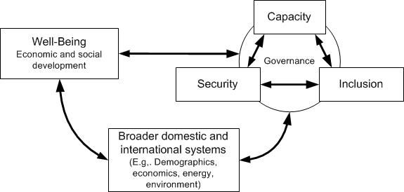
The conceptual foundation for the representation of governance in IFs owes much to an analysis of the evolution of governance in countries around the world over several centuries. That analysis (see Chapter 1 of the Strengthening Governance Globally volume by Hughes et al. 2014) identified three dimensions of governance: security, capacity, and inclusion. It traced them over time and noted their largely sequential unfolding for currently developed countries and their currently simultaneous progression in many lower-income countries.
The three dimensions interact closely and bi-directionally with each other. They also interact bi-directionally with broader human development systems. The level of well-being, often captured quantitatively by GDP per capita or the more inclusive human development index, may be especially important, but is hardly alone in helping drive forward advance in governance; for instance, the age structures of populations and economic structures also interact with governance patterns both indirectly through well-being and directly.
The conceptualization of governance further divides each of the three primary dimensions into two sub-dimensions partly based on the desire to quantify them historically and to facilitate forecasting. For security those are the probability of intrastate conflict and the general level of country performance and risk. The two sub-dimensions of capacity are the ability to raise revenue and the effective use of it and the other tools of government—that is, the competence or quality of governance. We use corruption (that is, control of it) as a proxy for such competence. The first sub-dimension of inclusion is the level of formal democratization, typically assessed in terms of competitive elections. More broadly democratization involves inclusion of population groupings across lines such as ethnicity, religion, sex, and age; we use gender equity as a proxy for the second dimension.
See Hughes et al. (2014), especially Chapter 4, for more background on the development of the governance representations of IFs than this documentation provides. See also Hughes (2002) for earlier and/or complementary work in IFs on socio-political representations (domestic and international); for example, here we do not discuss the formulations for power, interstate threat, and conflict, but that is available in documentation on the International Political model of the IFs system. Finally, we not provide here the important information about the forward linkages of governance to other elements of IFs, including to the production function of the economic model and to the broader financial flows of the social accounting matrix representation. See documentation on the economic model for that information.
Structure and Agent System: Governance
System/Subsystem
|
Governance
|
Organizing Structure
|
Three dimensions with two sub-dimensions each; highly interactive, bi-directional relationships among dimensions and with socio-economic development, demographics, and economics
|
Stocks
|
Socio-economic development levels (e.g. level of education, gender relationships, size of the economy); past patterns of governance; also cultural patterns are a stock
|
Flows
|
Government spending on human capital, infrastructure, development generally; accretion of changes in governance over time
|
Key Aggregate Relationships (illustrative, not comprehensive)
|
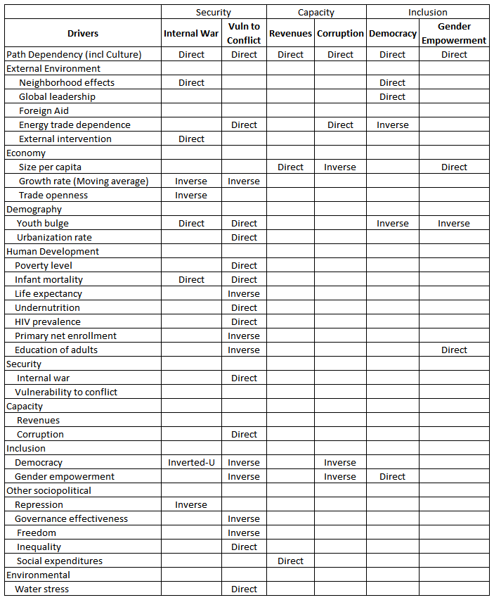
Probability of intrastate conflict is a function of past conflict, neighborhood effects, economic growth rate (inverse), trade openness (inverse), youth bulge, infant mortality, democracy (inverted-U), state repression (inverse), and external intervention. Vulnerability to intrastate conflict is a function of past intrastate conflict, energy trade dependence (as a proxy for broader natural resource dependence), economic growth rate (inverse), youth bulge, urbanization rate, poverty level, infant mortality, life expectancy (inverse) undernutrition, HIV prevalence, primary net enrollment (inverse), adult education levels (inverse), corruption, democracy (inverse), gender empowerment (inverse), governance effectiveness (inverse), freedom (inverse), inequality, and water stress Government revenues are a function of past revenue as percentage of GDP, GDP per capita, and social expenditures (that is, inversely to fiscal balance). Corruption is a function of past corruption level, GDP per capita (inverse), energy trade dependence, democracy (inverse), gender empowerment (inverse), and probability of intrastate conflict. Democracy is a function of past democracy level, youth bulge (inverse), and gender empowerment. Gender empowerment is a function of past gender empowerment level, GDP per capita, youth bulge (inverse), and primary net enrollment.
|
Key Agent-Class Behavior Relationships (illustrative, not comprehensive)
|
Social sub-group relationships, especially historical conflict patterns and gender relationships; government revenue and expenditure
|
Dominant Relations: Governance
The drivers of change on each dimension and sub-dimension of governance range widely. A quick summary (see also the table below) is that:
- Probability of intrastate conflict is a function of past conflict, neighborhood effects, economic growth rate (inverse), trade openness (inverse), youth bulge, infant mortality, democracy (inverted-U), state repression (inverse), and external intervention (inverse).
- Vulnerability to intrastate conflict is a function of energy trade dependence, economic growth rate (inverse), urbanization rate, poverty level, infant mortality, undernutrition, HIV prevalence, primary net enrollment (inverse), intrastate conflict probability, corruption, democracy (inverse), governance effectiveness (inverse), freedom (inverse), and water stress.
- Government revenues are a function of past revenue as percentage of GDP, GDP per capita, and fiscal balance (inverse).
- Corruption is a function of past corruption level, GDP per capita (inverse), energy trade dependence, democracy (inverse), gender empowerment (inverse), and probability of intrastate conflict.
- Democracy is a function of past democracy level, economic growth rate (inverse), youth bulge (inverse), and gender empowerment.
- Gender empowerment is a function of past gender empowerment level, GDP per capita, youth bulge (inverse), and primary net enrollment.
There are some general insights with respect to elaboration of the formulations (equations and algorithms) that drive change on each dimension and sub-dimension of governance:
- In almost each case there are path dependencies that supplement the basic relationships—social change has considerable inertia.
- The driving and driven variables clearly constitute a complex syndrome of mutually interdependent developmental interactions, not a simple causal sequence.
- There is a tendency for the dimensions of governance traditionally developing later to feed back to earlier ones, notably for inclusion to affect capacity via reduced corruption and also for inclusion and capacity to reduce the probability of internal conflict.
- Behaviorally, the bi-directional structures suggest the possibility that reinforcing processes may accelerate as governance strengthens, setting up a kind of tipping from one equilibrium to another; vicious cycles of deterioration would also be possible.
For detailed discussion of the model's causal dynamics, see the discussions of flow charts (block diagrams) and equations.
Governance Flow Charts
Overview
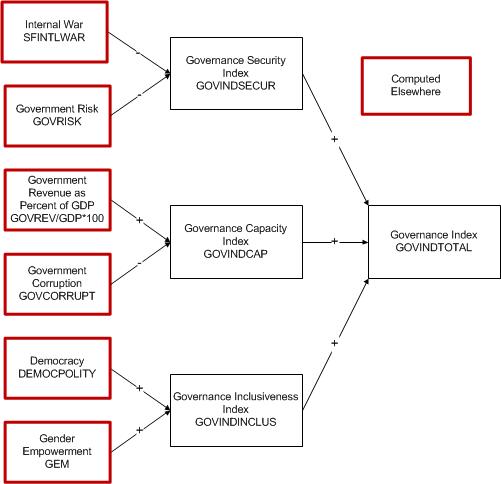
We can show and briefly describe a block diagram for each of the three dimensions of governance and the two sub-dimensions of those: security (probability of intrastate or internal war and risk of conflict); capacity (ability to mobilize revenues and the effectiveness of their use); inclusiveness (formal democracy and broader inclusiveness, using gender empowerment as a proxy).
Please click on the links below to access these topics.
Security
Internal War
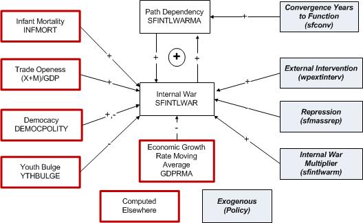
Internal or intrastate war (SFINTLWAR) is heavily determined by a moving average of a society's past experience with such conflict (SFINTLWARMA) in what is a positive feedback system. The probability of such conflict will, however, typically converge to that determined by more basic underlying drivers, and the user can control the speed of such convergence by specifying the years to convergence (sfconv ).
The major driving variables in a statistical estimation are the level of infant mortality (INFMORT) as a proxy for quality of government performance and trade openness or exports (X) plus imports (M) as a share of GDP. In addition democracy level (DEMOCPOLITY) enters in a non-linear and algorithmic fashion, as do youth bulge (YTHBULGE) and a moving average of economic growth rate (GDPRMA).
Although less often used and turned off in the Base Case scenario, external interventions (wpextinterv ) and mass repression (sfmassrep ) can cause or at least temporarily dampen internal war, respectively.
Finally, the user can multiply resultant endogenous values of internal war (sfintlwarm ) in order to generate user-controlled scenarios.
The IFs system also includes a representation of instability short of internal war (SFINSTABALL and SFINSTABMAG), linking them to the category of abrupt regime change in the classification developed by Ted Robert Gurr and used by the Political Instability Task Force. The forecasting representation was developed before the revision and update of that for internal war, however, and we recommend less attention to it until its own revision is done.
Vulnerability and Risk of Conflict
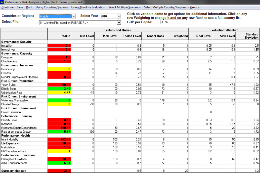
The IFs treatment of societal/governance performance risk and related vulnerability to conflict does not involve an estimated formulation. Instead, like other such efforts, it involves the creation of an index. The figure below, a screen capture of the form (reached via Specialized Displays) uses variables related both directly to governance and to performance. A specialized Help topic on this form is available.
Although many users will be interested in the rankings of countries (see the Global Rank column for ranks on individual variables and the summary measure for overall, variable-weighted rank), others will be interested in the summary value across all variables, shown at the bottom of the first column. Those values are also available in the model as the variable named government risk (GOVRISK).
Capacity
Government Revenues
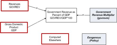
The ability to raise government revenues (GOVREV as a share of GDP) is one of the dimensions of capacity in governance. Its basic calculation is a very simple ratio. The key drivers of GOVREV, however, documented elsewhere, are very complex. For instance, GOVREV is responsive in an equilibration process to government expenditures, both transfer payments and direct government expenditures in categories such as military, health, education, and infrastructure, as well as to external revenues, notably foreign aid receipts.
Effectiveness of Government
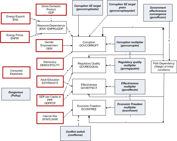
The central measure of governance effectiveness in Hughes et al. (2014) was defined to be corruption or GOVCORRUPT (actually the absence thereof, or level of transparency). The model computes several additional measures of effectiveness or ca
pacity, however, including regulatory quality (REGQUALITY) and effectiveness (GOVEFFECT), both related to the World Bank's World Governance Indicator project (Kaufmann, Kraay, and Mastruzzi 2010). In addition, many analysts point to the level of economic freedom (ECONFREE) or liberalization as a measure of effectiveness, in spite of considerable debate around their doing so.
Among the drivers of governance corruption is resource dependence, for which we use as a proxy the value of energy exports (ENX) at energy prices (ENPRI) as a share of GDP. Energy exports tend to me the largest such category globally. Further drivers are the extent of gender empowerment (GEM) and the level of democracy (DEMOCPOLITY), both of which indicate the extent of inclusiveness but which make independent statistical contributions to corruption level.
The drivers do not, of course, fully determine the level of corruption and there is much historical path dependence in societies related to other variables. The user can control the speed of elimination of such dependence and therefore of convergence to the basic formulation with a conversion years parameter (goveffconv ).
There are times when the user will wish to introduce normatively controlled target values for corruption. One approach is use of the "brute force" multiplier on corruption (govcorruptm ). A second approach involves the specification of target values relative to a function of the key drivers estimated cross-sectionally across countries. This second approach allows, for instance, the specification of a target level 1 or 2 standard errors (SE) above the level expected of a country given those drivers. The SE target parameter is govcorruptsetar and the govcorruptseyrtar carries the years to achieve the target. There are similar control parameters (not shown the diagram) for regulatory quality (govregqualsetar and govreqqualseyrtar ) and for effectiveness (goveffectsetar and goveffectseyrtar ), but not for economic freedom.
Theoretically, internal war (SFINTLWAR) could affect all of the capacity variables, but the only linkage identified in IFs is that to economic freedom. Setting the control switch (confforsw ) to 1 turns on that impact.
Inclusiveness
Democracy
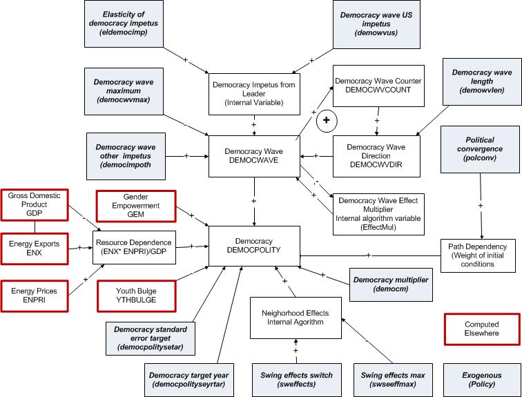
Three variables dominate the forecasting formulation for democracy (DEMOCPOLITY): the gender empowerment measure (GEM) as a measure of broad social inclusion (positive linkage), the youth bulge (YTHBULGE) as an indicator of the age structure of society (negative linkage), and the dependence of the country on raw materials exports, a negative linkage using energy export share (ENX) times energy prices (ENPRI) as a share of the GDP as a proxy. An exogenous multiplier (democm ) allows the user to directly manipulate the democracy level.
Two other variables can affect the democracy level but are turned off in the Base Case and will seldom be used. The first is the neighborhood effects of swing states in a regional neighborhood (e.g. Russia among former states of the Soviet Union). The swing states effect switch (sweffects ) turns it on when set to 1.
The more complicated additional factor is that of democracy waves (DEMOCWAVE). Relative to the initial condition a democracy wave can add or subtract democracy to the basic formulation's calculation of it (an algorithm based on historical experience allows upward swings to be larger than downward ones depending on EffectMul). The basic magnitude of increments depends of an exogenous specification of the impetus provided to democracy by the leading power (democwvus ) and by other powers (democimpoth ), the former's impact controlled by an elasticity (eldemocimp ). Because waves rise and ebb, another parameter controls the length (democlen ) and still another sets the maximum rise (democwvmax ). A counter keeps track of the running and receding of a wave (DEMOCWVCOUNT) and a pointer keeps track of the direction its operation (DEMOCWVDIR); these two parameters are linked with the magnitude of the wave in a positive loop.
The calculation from the basic formulation, before the addition of wave and swing state or neighborhood effects, can also be overridden by the use of external targeting directed by specifications of standard error targets relative to the formulation (democpolitysetar ) to be achieved by a target year (democpolityseyrtar ).
Gender Empowerment and Freedom
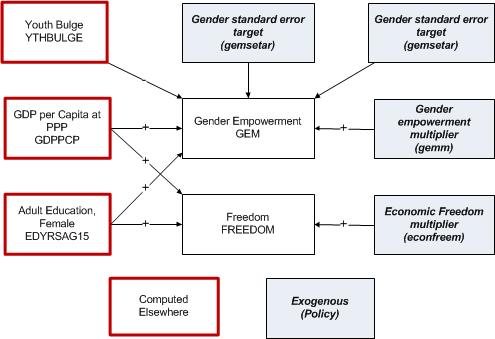
Gender empowerment (GEM), a broader measure of inclusion, joins democracy as the secon
d key measure of governance inclusiveness. Its three basic drivers are youth bulge size (YTHBULGE), GDP per capita as purchasing power parity (GDPPCP), and the years of formal education obtained by female adults (EDYRSAG15).
A user can control the progression of gender empowerment with a simple multiplier (gemm ) or via setting a target value for it movement to some number of standard errors above or below a cross-sectionally estimated function (gemsetar ) across a set number of years (gemseyrtar ).
Although IFs uses the Polity measure of democracy (DEMOCPOLITY) as its main measure of more formal, electoral inclusion, Freedom House's freedom measure (FREEDOM) is a logical alternative and the second of that measure's sub-dimensions, civil liberties, is a more inclusive measure. We therefore compute it also, using again GDP per capita and educational years (of all adults, not just females) as drivers. And there is a brute force multiplier for it also (freedomm ). There is no SE targeting mechanism in place for the freedom variable.
Aggregate Governance Indicators
The major way of exploring the possible future of the three dimensions of governance is separately to use the two variables that represent each. But it is also useful to have more aggregate indices, first for each dimension and also across the three.
The governance security index (GOVINDSECUR) is computed as an unweighted average of internal war probability (SFINTLWAR) and governance/society performance risk (GOVRISK). Similarly, the governance capacity index (GOINDCAP) is an unweighted average of government revenue (GOVREV) as a portion of GDP and government corruption, while the governance inclusion index (GOVINCLIND) averages democracy (DEMOCPOLITY) and gender empowerment (GEM). The overall governance index (GOVINDTOTAL) is a simple average of those across dimensions.
In reality, creating the indices for each dimension requires some attention to scaling issues and valence. See the description of the equations for details.
Life Conditions and the Human Development Index
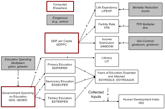
The condition of individuals and society are both the ultimate focus of governance and the font of it. The IFs system computes many of the relevant variables across its various models. It also aggregates a number of those into the widely used Human Development Index (HDI), based on heath (life expectancy), education or knowledge (both expectations for youth and attainment for adults), and GDP per capita.
Social Values and Cultural Evolution
Understanding societies fully requires going even more deeply than their governance
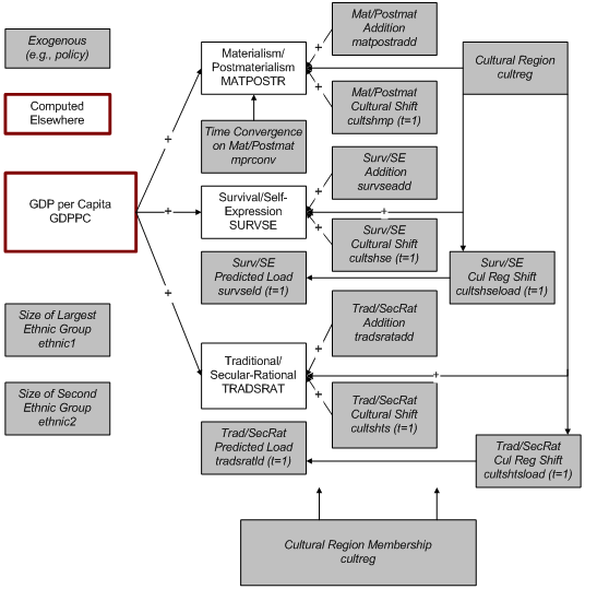
and social conditions in order to look at the values and cultural foundations. IFs computes change in three cultural dimensions identified by the World Values Survey (Inglehart 1997). Those are dimensions of materialism/post-materialism, survival/self-expression, and traditional/secular-rational values.
Inglehart has identified large cultural regions that have substantially different patterns on these value dimensions and IFs represents those regions, using them to compute shifts in value patterns specific to them.
Levels on the three cultural dimensions are predicted not only for the country/regional populations as a whole, but in each of 6 age cohorts. Not shown in the flow chart is the option, controlled by the parameter "wvsagesw ," of computing country/region change over time in the three dimensions by functions for each cohort (value of wvsagesw = 1) or by computing change only in the first cohort and then advancing that through time (value of wvsagesw = 2).
The model uses country-specific data from the World Values Survey project to compute a variety of parameters in the first year by cultural region (English-speaking, Orthodox, Islamic, etc.). The key parameters for the model user are the three country/region-specific additive factors on each value/cultural dimension (matpostradd , etc.).
Finally, the model contains data on the size (percentage of population) of the two largest ethnic/cultural groupings. At this point these parameters have no forward linkages to other variables in the model. <header><hgroup>
Governance Equations
</hgroup></header>
Overview
Like the block diagrams for governance in IFs, the equations fall into the categories of the three dimensions (security, capacity, and inclusion), with detail for each of two sub-dimensions on each. <header><hgroup>
Governance Security Dimension
</hgroup></header>
Overview
IFs represents two different types of measures related to domestic conflict and security. The first has roots in the work of the Political Instability Task Force (PITF); see Esty et al. (1998) and Goldstone et al. (2010). The PITF database allows us to see the actual pattern of conflict in countries over time and to use that historical conflict pattern to compute an initial probability of conflict. The second type of measure includes indices of vulnerability to conflict, generally presented in terms of rankings of countries with respect to their vulnerability (see Chapter 2 of Hughes et al. 2014, especially Box 2.3). Because these indices are not rooted as solidly in past conflict patterns, we cannot interpret their values or the rankings based on them as probabilities of conflict, but rather as propensities for conflict (and as indicators more generally of country performance and risk).
In order to establish forecasting approaches for both types of measures within IFs, we looked to earlier work (see Chapter 3 of Chapter 2 of Hughes et al. 2014), did our own statistical analysis to create an underlying base formulation for overt conflict probability, and augmented the basic approach via more algorithmic elements—algorithms or logical procedures, like recipes, help guide forecasting through steps that analytical functions cannot easily represent. The algorithmic elements are tied in part to our efforts to fit the IFs forecasting approach at least relatively well to historical data from 1960 through 2010. Chapter 4 of Hughes et al. 2014 elaborates more fully the development process for the representation of security provided in this Help system.
For more, please click on the links below. <section id="main"><section id="mainContent"><header><hgroup>
Equations: Internal Conflict or War Probability
</hgroup></header> The PITF defined state failure in terms of four different types of events (with specific magnitude thresholds)—namely, adverse regime change (such as coups), revolutionary wars, ethnic wars, and genocides or politicides (Esty et al. 1998). On the recommendation of Ted Robert Gurr, one of the founding fathers of the PITF data project and approach, IFs builds two categories of insecurity from those four types: instability (adverse regime change); and internal war (combining revolutionary war, ethnic war, and genocide or politicide).
Presence of any one of the three types of war, either as an initiation or continuation, leads us to code a country as 1; otherwise we code the country as 0. This distinction between instability and internal war helps differentiate among what Easton (1965) identified as regime, state, and polity levels within the sociopolitical system, by at least differentiating the regime level (where adverse regime changes occur) from the more fundamental state and polity levels. The forces of change and generally the extent of violence around change differ significantly at these different levels.
Looking at the historical patterns of conflict in global regions across time (see Chapter 4 of Hughes et al. 2014) and doing our own statistical analysis it is clear that the "usual suspect" variables will not explain those patterns, and that in many cases they cannot therefore be very effective in forecasting. We found:
- Normed infant mortality proves statistically interesting, being associated with (explaining or being explained by, using a second-order polynomial form) about 12 percent of cross-country variation in intrastate conflict in the most recent data-year (8.9 percent in panel analysis across the 1960–2000 period). Thus in forecasting it may help us understand general propensity for conflict, but its slow variation over time means it cannot possibly explain the big historical surges of warfare within regions and their country members.
- Trade openness (which we define as the sum of exports and imports as a percentage of GDP) can be helpful in understanding variations in conflict and does vary within countries more rapidly than infant mortality. In cross-sectional analysis with most recent data, infant mortality and trade openness (inverse relationship) together account for 15 percent of the variation in intrastate conflict (trade openness itself is associated with 11 percent of the variance within intrastate conflict in a logarithmic formulation). Moreover, its increase coincides with the reduction of conflict historically within the countries of East Asia. But openness perversely increased over time in South Asia as intrastate conflict also rose. And its statistical power is good but not great. Again, causality could run in either direction or be a spurious result of a third variable; for instance, the end of Indochina wars and a change in economic policy in socialist countries could have led to greater trade there.
- Factionalism, which can have many bases, including ethnicity or the intensity of feelings around ethnicity, is of surprisingly little use in forecasting. Most underlying social divisions change very slowly over time. Although intensity of factionalism around those divisions may change much more rapidly (for instance, as "conflict entrepreneurs" inflame passions), we arguably cannot anticipate when that might happen. Nor do we believe we can we anticipate changes in other potential ideational drivers, such as ideologies. Further, historical measurement of change in factionalism risks using conflict as a proxy, thereby creating the danger that correlations between it and conflict are simply a tautological artifact of that measurement. Finally, our own analysis of various measures of ethnic and/or religious factionalism and intrastate conflict suggests lower relationship than we expected.
- Youth bulges are a potentially more useful driver in forecasting because our demographic forecasts are stronger than those of variables like factionalism or even trade openness, and because demographic structures exhibit clear and non-monotonic variation over time. There were many bulges in East Asia during the 1970s, as there have been many recently in South Asia and as there are today in the Middle East and North Africa. In cross-sectional analysis of recent data, a linear relationship with youth bulge size accounts for 7 percent of the variation in conflict (in panel analysis since 1960, however, only 3.5 percent).
- Consistent with studies that have found anocracy rather than autocracy primarily related to conflict, the relationship of measures of regime type with conflict has an inverted U-shaped character. Using a third-order polynomial, we found that the Polity measure of regime type explains 4 percent of variation in recent intrastate war. The Freedom House measure (see http://www.freedomhouse.org/) actually explains 10 percent, but we used the Polity Project measure (see http://www.systemicpeace.org/polity/polity4.htm) because it is a purer measure of political democracy (rather than civil liberties as well) and because it is our primary measure of regime in forecasting.
- Downturns in economic growth rates preceded the collapse of communism in Europe and Central Asia, the rise of internal conflict in both Latin America and the Middle East in the 1980s, and more recently the events of the Arab Spring. Analysis of the magnitude of downturn required to generate conflict and the lag between downturn and conflict is complex. We found, through experimentation directed at fitting historical conflict patterns (running IFs against historical patterns since 1960), that a 1.0 percent drop in a moving average of economic growth (carrying 60 percent of the moving average forward) is associated with a 0.04 point increase on a 0-1 scale for the rate of internal war.
- Conflict begets conflict. We found, again through historical analysis, a 60 percent carryover of past conflict levels to current ones.
For IFs forecasting, we conceptualize and operationalize intrastate war not as a 0 or 1 outcome as in the data (no war or war), but as a probability of conflict in any country-year. We initialize country probabilities at the beginning of a forecast horizon with average conflict rates across the preceding 20 years. The development of our own basic forecasting formulation for these probabilities involved not just literature and statistical analysis, but testing of the formulation in runs of the model from 1960 through 2010 and comparisons of our historical forecasts with the data on intrastate war. We let the historical forecasts run without the frequently used annual adjustment/correction by the historical conflict data for the full 50 years. We experimented with a number of algorithmic elements in order to improve the historical fit. This analysis yielded the following basic formulation:
http://www.du.edu/ifs/help/media/images/gov-module-updated/goveq_1.png
SFINTLWAR=probability of internal war or state failure
INFMOR=infant mortality, normed globally
TRADEOPEN=trade openness ratio
X=exports in billion dollars
M=imports in billion dollars
GDP=gross domestic product in billion dollars
POLITYDEMOC=Polity’s 21-point scale of democracy; asymmetrical curvilinear relationship with a peak at 9 and a sharper fall than rise
YTHBULGE=population age 15–29 as a portion of all adults; algorithmic adjustment with GDP/capita explained in text
GDPRMA=gross domestic product growth rate, algorithmic moving average carrying forward 60 percent past year’s value; algorithmic adjustment with GDP/capita explained in text; inverse relationship
SFINTLWARMA=moving average of past internal war probability (i.e., carrying forward past forecast values, not past data values)
sfintlwarm=an exogenous multiplier for scenario analysis
Algorithm on regional contagion explained in text
R-squared = 0.22 in 50-year historical simulation without annual correction (see text for elaboration)
Our historical and extended analytical explorations of the core statistical formulation with infant mortality and trade openness led us to make a number of algorithmic changes to it in creating our basic formulation. We found that $18,000 per capita (in 2005 dollars at PPP) is a point above which economic downturns and youth bulges tend not to increase the probability of internal war, so we greatly dampened the affects of both of those variables above that level. We also found it important to add a regional contagion effect; courtesy of data provided by Paul Diehl we combined three of the Correlates of War Project distance categories (contiguous, less than 12 miles separation, and less than 24 miles separation) and added 0.1 to conflict probability for a country for each neighbor with computed conflict probability of its own above 0.2— because of conflict carryover across time, this algorithm can also lead to a positive feedback loop of neighborhood contagion.
We further found that the intrastate war formulation is sensitive to actual GDP levels, not just because of the growth rate term, but because within the broader IFs system GDP per capita also affects the endogenously calculated youth bulge and democracy variables (we will return to discussion of the latter). To deal with this sensitivity, we forced the IFs historical base to be historically accurate with respect to GDP growth—otherwise the entire historical forecast of IFs after 1960 was endogenously determined in recursive annual calculation only by initial conditions and formulations rather than with annual corrective terms often used in historical validation exercises.
This basic initial formulation generated a pattern of historical forecasts (which can be generated using the file HistoricalNoMassRepOrExtInterv.sce) of intrastate warfare probabilities that showed some of the characteristics of the historical data, including a peak for the Middle East and North Africa in the 1980s and one for developing Europe and Central Asia in the early 1990s (both related to growth downturns). Visual comparison quickly suggested, however, that the overall pattern was not a good historical fit. In particular, the bulges of conflict in East Asia in the early years and of South Asia more recently were missing; in addition, because of the infant mortality and economic growth terms, the model generated a bulge of conflict within Africa in the early 1980s (when growth and social advance was very weak) that did not appear in the data. Moreover, statistically, the forecasts correlated at the region level with data across the 1960-2010 time period with only a 0.19 R-squared level.
We therefore explored the bases of the historical patterns further, and concluded that additional factors were missing. One is the extreme or totalitarian repression that lowered conflict in developing Europe and Central Asia until about the time of General Secretary Mikhail Gorbachev; we added a repression parameter (wpextinterv) for exogenous manipulation. More controversially perhaps, we also found it necessary to extend the suppression of conflict to sub-Saharan Africa in the middle period of the historical run; the underlying assumption is that the domestic prestige and power of liberation movement leaders, backed by their domestic and superpower supporters, helped dampen conflict significantly in the face of poor, and even deteriorating, domestic economic and social conditions.
A second type of factor missing in our basic statistical analysis is external interventions, such as those of the U.S. in Southeast Asia in the 1960s and those of the former USSR and then the U.S. in South Asia after 1980; we added another exogenous parameter (sfmassrep) to represent such interventions.
Although still not a terribly strong match to actual history, this revised historical forecast some remarkable similarities, including the initially high level of conflict in East Asia and the Pacific and a relatively high rate for South Asia in recent decades. The adjusted R-squared rises to 0.61 from 0.19 (before the addition of the repression and intervention variables). The major problems that remained in our historical forecast include the generation by the model of too much conflict for Latin America and the Caribbean in the 1980s, when economic and social conditions in that region deteriorated significantly; and the relatively high levels of conflict in sub-Saharan Africa beyond the end of the Cold War, again associated in our forecast with a combination of absolute and relative deterioration in socioeconomic conditions of many countries. Thus the additional parameters may be useful in scenario analysis.
It is possible that our relatively high historical forecasts for conflict in post-Cold War sub-Saharan Africa, even after formulation enhancements, may reflect the remaining omission of yet another systemic variable, namely regional and global efforts to dampen conflict there. There is no parameter to represent that variable, but the user can use the overall multiplier (sfintlwarm ) in scenario analysis. <header><hgroup>
Equations: Political Stability/Instability
</hgroup></header> The State Failure project has analyzed the propensity for different types of state failures within countries, including those associated with revolution, ethnic conflict, genocide-politicide, and abrupt regime change (using categories and data pioneered by Ted Robert Gurr. Upon the advice of Gurr, IFs groups the first three as internal war and the last as political instability. The model formulations for political instability are older and less well developed than those for internal war; we therefore recommend focus on internal war. Nonetheless, we document the approach to instability here.
The extensive database of the project includes many measures of failure. IFs has variables representing the probability of the first year or a continuing year of instability (SFINSTABALL) and the magnitude of a first year or continuing event (SFINSTABMAG).
Using data from the State Failure project, formulations were estimated for each variable using up to five independent variables that exist in the IFs model: democracy as measured on the Polity scale (DEMOCPOLITY), infant mortality (INFMOR) relative to the global average (WINFMOR), trade openness as indicated by exports (X) plus imports (M) as a percentage of GDP, GDP per capita at purchasing power parity (GDPPCP), and the average number of years of education of the population at least 25 years old (EDYRSAG25). The first three of these terms were used because of the state failure project findings of their importance and the last two were introduced because they were found to have very considerable predictive power with historic data.
The IFs project developed an analytic function capability for functions with multiple independent variables that allows the user to change the parameters of the function freely within the modeling system. The default values seldom draw upon more than 2-3 of the independent variables, because of the high correlation among many of them. Those interested in the empirical analysis should look to a project document (Hughes 2002) prepared for the CIA's Strategic Assessment Group (SAG), or to the model for the default values.
One additional formulation issue grows out of the fact that the initial values predicted for countries or regions by the six estimated equations are almost invariably somewhat different, and sometimes quite different than the empirical rate of failure. There may well be additional variables, some perhaps country-specific, that determine the empirical experience, and it is somewhat unfortunate to lose that information. Therefore the model computes three different forecasts of the six variables, depending on the user's specification of a state failure history use parameter (sfusehist). If the value is 0, forecasts are based on predictive equations only. The equation below illustrates the formulation. The analytic function obviously handles various formulations including linear and logarithmic.
http://www.du.edu/ifs/help/media/images/gov-module-updated/goveq_2.png
If the value of the sfusehist parameter is 1, the historical values determine the initial level for forecasting, and the predictive functions are used to change that level over time. Again the equation is illustrative.
http://www.du.edu/ifs/help/media/images/gov-module-updated/goveq_3.png
If the value of the sfusehist parameter is 2, the historical values determine the initial level for forecasting, the predictive functions are used to change the level over time, and the forecast values converge over time to the predictive ones, gradually eliminating the influence of the country-specific empirical base. That is, the second formulation above converges linearly towards the first over years specified by a parameter (polconv), using the CONVERGE function of IFs.
http://www.du.edu/ifs/help/media/images/gov-module-updated/goveq_5.png <header><hgroup>
Equations: Vulnerability to Conflict (and Performance Risk Analysis)
</hgroup></header> The second approach to analyzing risk of violent internal conflict (and broader country risks) involves the creation of indices that tend to rank states according to generalized performance. The projects creating such indices—variously referred to as measures of state fragility, state weakness, political instability, or failed states—most often do not intend to convey a probability of violent internal conflict. Rather they try to suggest greater or lower propensities for conflict as well as broader country risk, for instance that which foreign investors might face with respect to socioeconomic conditions. .
Generally, these indices combine variables in four categories: social, political, economic, and security. Developers may supplement variables that mostly focus on the average values for countries with select variables focusing on distribution (such as the Gini index). They commonly weight variables within categories equally and/or weight the categories equally when aggregating them to final index values. While individual variables have theoretical and empirical links to conflict or lack of security, such simple combination of large numbers of highly intercorrelated variables into a formulation of conflict vulnerability is very difficult to interpret. Moreover, because reports generally present an index with no simple interpretation of scale, analysts focus heavily on rankings of countries.
The IFs project has created its own Performance Risk Index (see variable GOVRISK) along the lines of these approaches, and for the purposes of forecasting has uniquely made it responsive to endogenous long-term change in the underlying variables. Like those of other projects, the IFs measure draws upon social, political, economic, and security variables, but we impose a different conceptual or analytical structure on them (see the example risk analysis form provided here). We divide the variables of the index into three general categories: governance, (deep) risk drivers, and performance. We further divide the governance variables into our three dimensions of security, capacity and inclusion, the deep risk factors into demographic, environmental, and international categories, and the performance factors into economic, health, and education categories. </section></section>
