Population: Difference between revisions
StellahKwasi (talk | contribs) No edit summary |
StellahKwasi (talk | contribs) No edit summary |
||
| Line 1: | Line 1: | ||
= Crude death rate (CDR) = | = <span style="font-size:smaller">Crude death rate (CDR)<br/></span> = | ||
From population.bas: | <span style="font-size:smaller">From population.bas:</span> | ||
"There are three numbers that capture fertility: TFR, CBR, the fertility distribution. There are three numbers that caputure mortality: LIFEXP, CDR, mortality distribution. They will not be completely compatible. The distributions must be used to handle cohort dynamics. But they may not be available for all countries (e.g. Taiwan, Palestine), whereas the others are. For many years we used CBR and CDR to adjust the distributions and then calculated TFR and LIFEXP from them. Over time, TFR and LIFEXP have become the key variables that dynamically drive the population model, and good data are now available. We have therefore switched over to them as the bases for initial conditions of the model, calculating CBR and CDR from them, giving us also POPR. | <span style="font-size:smaller">"There are three numbers that capture fertility: TFR, CBR, the fertility distribution. There are three numbers that caputure mortality: LIFEXP, CDR, mortality distribution. They will not be completely compatible. The distributions must be used to handle cohort dynamics. But they may not be available for all countries (e.g. Taiwan, Palestine), whereas the others are. For many years we used CBR and CDR to adjust the distributions and then calculated TFR and LIFEXP from them. Over time, TFR and LIFEXP have become the key variables that dynamically drive the population model, and good data are now available. We have therefore switched over to them as the bases for initial conditions of the model, calculating CBR and CDR from them, giving us also POPR.</span> | ||
== Demography/Population == | == <span style="font-size:smaller">Demography/Population</span> == | ||
=== Overview === | === <span style="font-size:smaller">Overview</span> === | ||
The most recent and complete demographic model documentation is available on Pardee's [http://pardee.du.edu/ifs-population-model-documentation website]. Although the text in this interactive system is, for some IFs models, often significantly out of date, you may still find the basic description useful to you. | <span style="font-size:smaller">The most recent and complete demographic model documentation is available on Pardee's [http://pardee.du.edu/ifs-population-model-documentation website]. Although the text in this interactive system is, for some IFs models, often significantly out of date, you may still find the basic description useful to you.</span> | ||
The population sub-model of IFs uses the cohort component analysis approach of many population models, including the studies done by the United Nations (United Nations, 1956 and 1977). The structure of the IFs population model drew initially on the World Integrated Model (WIM) or the second generation Mesarovic-Pestel Model (Hughes, 1980), but has changed much over time. In particular, José Solórzano and Randall Kuhn have made many contributions to its development. | <span style="font-size:smaller">The population sub-model of IFs uses the cohort component analysis approach of many population models, including the studies done by the United Nations (United Nations, 1956 and 1977). The structure of the IFs population model drew initially on the World Integrated Model (WIM) or the second generation Mesarovic-Pestel Model (Hughes, 1980), but has changed much over time. In particular, José Solórzano and Randall Kuhn have made many contributions to its development.</span> | ||
The approach relies upon age, fertility, and mortality distributions for each country/region with 22 cohorts: one for infants, 20 of five-year size, and one for all individuals of age 100 or older. A major advantage of five-year cohorts is that data sources generally present demographic data in that form. Ideally, however, the cohort size should correspond to the model time step so as to avoid "numerical diffusion," the propagation of change from a five-year cohort to an adjoining cohort in a single year. To prevent such numerical diffusion, IFs actually runs an age distribution with 100 single-year cohorts and advances that over time, collapsing to 22 cohorts only for the calculations of births and deaths. | <span style="font-size:smaller">The approach relies upon age, fertility, and mortality distributions for each country/region with 22 cohorts: one for infants, 20 of five-year size, and one for all individuals of age 100 or older. A major advantage of five-year cohorts is that data sources generally present demographic data in that form. Ideally, however, the cohort size should correspond to the model time step so as to avoid "numerical diffusion," the propagation of change from a five-year cohort to an adjoining cohort in a single year. To prevent such numerical diffusion, IFs actually runs an age distribution with 100 single-year cohorts and advances that over time, collapsing to 22 cohorts only for the calculations of births and deaths.</span> | ||
Because extensions of life expectancy are occurring steadily and there is at least the possibility of substantial breakthroughs, the IFs project has also created the option of extending the number of cohorts from 22 up to as many as 42 (allowing separate representation of age categories up to 200+). The capability is normally turned off, but instructions for turning on extended aging can be found [http://www.du.edu/ifs/help/understand/demography/flowcharts/ here]. | <span style="font-size:smaller">Because extensions of life expectancy are occurring steadily and there is at least the possibility of substantial breakthroughs, the IFs project has also created the option of extending the number of cohorts from 22 up to as many as 42 (allowing separate representation of age categories up to 200+). The capability is normally turned off, but instructions for turning on extended aging can be found [http://www.du.edu/ifs/help/understand/demography/flowcharts/ here].</span> | ||
== Structure and Agent System: Demographic == | == <span style="font-size:smaller">Structure and Agent System: Demographic</span> == | ||
{| class="tableGrid" style="width: 100%" cellspacing="0" cellpadding="5" border="0" | {| class="tableGrid" style="width: 100%" cellspacing="0" cellpadding="5" border="0" | ||
|- | |- | ||
| style="width: 50%" | <div>'''System/Subsystem'''<br/></div> | | style="width: 50%" | <div><span style="font-size:smaller">'''System/Subsystem'''<br/></span></div> | ||
| style="text-align: left; padding-left: 10px" align="center" | <div>Demographic</div> | | style="text-align: left; padding-left: 10px" align="center" | <div><span style="font-size:smaller">Demographic</span></div> | ||
|- | |- | ||
| style="text-align: left" | <div>'''Organizing Structure'''</div> | | style="text-align: left" | <div><span style="font-size:smaller">'''Organizing Structure'''</span></div> | ||
| style="text-align: left; padding-left: 10px" align="center" | <div>Cohort-component</div> | | style="text-align: left; padding-left: 10px" align="center" | <div><span style="font-size:smaller">Cohort-component</span></div> | ||
|- | |- | ||
| style="text-align: left" | <div>'''Stocks'''</div> | | style="text-align: left" | <div><span style="font-size:smaller">'''Stocks'''</span></div> | ||
| style="text-align: left; padding-left: 10px" align="center" | <div>Population by age-sex</div> | | style="text-align: left; padding-left: 10px" align="center" | <div><span style="font-size:smaller">Population by age-sex</span></div> | ||
|- | |- | ||
| style="text-align: left" | <div>'''Flows'''</div> | | style="text-align: left" | <div><span style="font-size:smaller">'''Flows'''</span></div> | ||
| style="text-align: left; padding-left: 10px" align="center" | <div>Birth, death, migration</div> | | style="text-align: left; padding-left: 10px" align="center" | <div><span style="font-size:smaller">Birth, death, migration</span></div> | ||
|- | |- | ||
| style="text-align: left" | <div>'''Key Aggregate ''' '''Relationships '''</div><div>(illustrative, not comprehensive)</div> | | style="text-align: left" | <div><span style="font-size:smaller">'''Key Aggregate ''' '''Relationships '''</span></div><div><span style="font-size:smaller">(illustrative, not comprehensive)</span></div> | ||
| style="text-align: left; padding-left: 10px" align="center" | <div>Life expectancy (from health model)</div> | | style="text-align: left; padding-left: 10px" align="center" | <div><span style="font-size:smaller">Life expectancy (from health model)</span></div> | ||
|- | |- | ||
| style="text-align: left" | <div style="text-align: left">'''Key Agent-Class Behavioral ''' '''Relationships'''</div><div style="text-align: left">(illustrative, not comprehensive)</div> | | style="text-align: left" | <div style="text-align: left"><span style="font-size:smaller">'''Key Agent-Class Behavioral ''' '''Relationships'''</span></div><div style="text-align: left"><span style="font-size:smaller">(illustrative, not comprehensive)</span></div> | ||
| style="text-align: left; padding-left: 10px" align="center" | | | style="text-align: left; padding-left: 10px" align="center" | | ||
Household fertility and migration | <span style="font-size:smaller">Household fertility and migration</span> | ||
|} | |} | ||
Humans as individuals within households interact in larger '''demographic systems or structures'''. The computer model should represent the behavior of such households, such as decisions to have children or to emigrate. And it should represent the larger demographic structures that incorporate the decisions of millions of such households. A typical approach to representing such demographic systems is through age-sex cohort distributions (see the figure below showing an example from the model). IFs also uses fertility and mortality distributions by age and sex and tracks migration across countries. | <span style="font-size:smaller">Humans as individuals within households interact in larger '''demographic systems or structures'''. The computer model should represent the behavior of such households, such as decisions to have children or to emigrate. And it should represent the larger demographic structures that incorporate the decisions of millions of such households. A typical approach to representing such demographic systems is through age-sex cohort distributions (see the figure below showing an example from the model). IFs also uses fertility and mortality distributions by age and sex and tracks migration across countries.</span> | ||
[[File:Pop1.png|right|Pop1.png]] | <span style="font-size:smaller">[[File:Pop1.png|right|Pop1.png]]</span> | ||
Demographers have widely accepted the representation of demographic systems and the development of demographic models with cohort-component structures. In fact, the United Nations, the U.S. Census Bureau, and the International Institute for Applied Systems Analysis (IIASA), pre-eminent demographic forecasting institutions, all use cohort-component modeling (O’Neill and Balk 2001) | <span style="font-size:smaller">Demographers have widely accepted the representation of demographic systems and the development of demographic models with cohort-component structures. In fact, the United Nations, the U.S. Census Bureau, and the International Institute for Applied Systems Analysis (IIASA), pre-eminent demographic forecasting institutions, all use cohort-component modeling (O’Neill and Balk 2001)</span> | ||
== Dominant Relations: Population == | == <span style="font-size:smaller">Dominant Relations: Population</span> == | ||
The dominant population (POP) equation is a simple addition of births (BIRTHS) at the bottom of the cohort distribution, subtraction of deaths (DEATHS) from each population cohort, and advance of people to the next cohort over time. | <span style="font-size:smaller"> The dominant population (POP) equation is a simple addition of births (BIRTHS) at the bottom of the cohort distribution, subtraction of deaths (DEATHS) from each population cohort, and advance of people to the next cohort over time.</span> | ||
The following key dynamics are directly linked to the Dominant Relations: | <span style="font-size:smaller">The following key dynamics are directly linked to the Dominant Relations:</span> | ||
Births are primarily a function of the total fertility rate (TFR), which in the longer term responds especially to education level of the adult population. The model user has direct control over TFR with a multiplier ('''''tfrm'' '''), but also much control for low fertility countries with a parameter specifying long-term stabilization level and lower boundary for fertility ('''''tfrmin'' '''). There is also a secular trend reduction in fertility (controlled by '''''ttfrr'' '''). | <span style="font-size:smaller">Births are primarily a function of the total fertility rate (TFR), which in the longer term responds especially to education level of the adult population. The model user has direct control over TFR with a multiplier ('''''tfrm'' '''), but also much control for low fertility countries with a parameter specifying long-term stabilization level and lower boundary for fertility ('''''tfrmin'' '''). There is also a secular trend reduction in fertility (controlled by '''''ttfrr'' ''').</span> | ||
Deaths are primarily a function of life expectancy (LIFEXP), itself computed within the IFs health model where, like fertility, it responds in the long run to adult education and also to GDP per capita and technology change. The model user has direct control over all deaths with a mortality multiplier ('''''mortm'' ''') and over those specific to a cause of health with an alternative multiplier ('''''hlmortm'' '''). There is also a secular trend reduction in mortality (controlled by '''''tmortr'' '''). | <span style="font-size:smaller">Deaths are primarily a function of life expectancy (LIFEXP), itself computed within the IFs health model where, like fertility, it responds in the long run to adult education and also to GDP per capita and technology change. The model user has direct control over all deaths with a mortality multiplier ('''''mortm'' ''') and over those specific to a cause of health with an alternative multiplier ('''''hlmortm'' '''). There is also a secular trend reduction in mortality (controlled by '''''tmortr'' ''').</span> | ||
<span>The larger demographic model in combination with the health model provides representation of and control over migration; the fertility impact of infant mortality and contraception use rates; and the mortality impact of many factors including undernutrition, smoking rates, and indoor air pollution from open burning of solid fuels.</span> | <span style="font-size:smaller">The larger demographic model in combination with the health model provides representation of and control over migration; the fertility impact of infant mortality and contraception use rates; and the mortality impact of many factors including undernutrition, smoking rates, and indoor air pollution from open burning of solid fuels.</span> | ||
== Demographic Flow Charts == | == <span style="font-size:smaller">Demographic Flow Charts</span> == | ||
=== Overview === | === <span style="font-size:smaller">Overview</span> === | ||
The demographic model represents the population of each geographic unit in terms of 22 cohorts (infants, five-year intervals up to age 99, and those aged 100 and older), separately for females and males. An age distribution records the population in each cohort and sex category. The sum across all cohorts in the age distribution and both sexes is the total population. A fertility distribution determines births, which are added to the bottom of the age distribution, while a mortality distribution determines deaths, which are subtracted from the appropriate cohort of the age distribution. | <span style="font-size:smaller">The demographic model represents the population of each geographic unit in terms of 22 cohorts (infants, five-year intervals up to age 99, and those aged 100 and older), separately for females and males. An age distribution records the population in each cohort and sex category. The sum across all cohorts in the age distribution and both sexes is the total population. A fertility distribution determines births, which are added to the bottom of the age distribution, while a mortality distribution determines deaths, which are subtracted from the appropriate cohort of the age distribution.</span> | ||
Those who might like to turn on the extension of age-cohort representation, to as many as 42, can do so by making changes in the IFsInit table of the IFsInit.mdb file. Specifically, the NCohorts field can be changed to as many cohorts as 42 and the NAges field can be changed up to 200. Registering these changes requires a rebuild of the Base Case (see documentation of Extended Features). | <span style="font-size:smaller">Those who might like to turn on the extension of age-cohort representation, to as many as 42, can do so by making changes in the IFsInit table of the IFsInit.mdb file. Specifically, the NCohorts field can be changed to as many cohorts as 42 and the NAges field can be changed up to 200. Registering these changes requires a rebuild of the Base Case (see documentation of Extended Features).</span> | ||
The population model is central to many broader dynamics of IFs. Two key feedback loops drive its own dynamics. The first is a positive feedback loop around fertility, linking population and births (causing population to drive exponentially upward if nothing else changes), while the second is a negative loop around mortality, linking population and deaths (causing population to decline). This second loop actually runs through the health model of IFs where deaths are computed (switching the control parameter '''''hlmodelsw'' ''' from 1 to 0 would, however, cause the model to revert to an earlier formulation in which life expectancy was computed as function of GDP per capita and controlled the death rate and deaths; it would turn off the health model's impact). A Malthusian variation of the negative feedback loop involving deaths may be of interest to those who believe that food supplies do or will play an important role in population dynamics (as they clearly do in countries with very low nutritional levels) by raising mortality rates, especially of children. See the topic on nutrition. Whether population rises or falls depends on the relative strength of those two loops. | <span style="font-size:smaller">The population model is central to many broader dynamics of IFs. Two key feedback loops drive its own dynamics. The first is a positive feedback loop around fertility, linking population and births (causing population to drive exponentially upward if nothing else changes), while the second is a negative loop around mortality, linking population and deaths (causing population to decline). This second loop actually runs through the health model of IFs where deaths are computed (switching the control parameter '''''hlmodelsw'' ''' from 1 to 0 would, however, cause the model to revert to an earlier formulation in which life expectancy was computed as function of GDP per capita and controlled the death rate and deaths; it would turn off the health model's impact). A Malthusian variation of the negative feedback loop involving deaths may be of interest to those who believe that food supplies do or will play an important role in population dynamics (as they clearly do in countries with very low nutritional levels) by raising mortality rates, especially of children. See the topic on nutrition. Whether population rises or falls depends on the relative strength of those two loops.</span> | ||
The easiest and most often used scenario handles for the population model are a multiplier on the total fertility rate (the number of children borne by an average woman in a lifetime), namely '''''tfrm'' ''', a multiplier on the total mortality rate, '''''mortm'' ''', and a multiplier on mortality by cause, '''''hlmortm'' '''. | <span style="font-size:smaller">The easiest and most often used scenario handles for the population model are a multiplier on the total fertility rate (the number of children borne by an average woman in a lifetime), namely '''''tfrm'' ''', a multiplier on the total mortality rate, '''''mortm'' ''', and a multiplier on mortality by cause, '''''hlmortm'' '''.</span> | ||
[[File:Pop2.png|right|Pop2.png]] | <span style="font-size:smaller">[[File:Pop2.png|right|Pop2.png]]</span> | ||
A large number of indicators are calculated in IFs from the age distribution: | <span style="font-size:smaller">A large number of indicators are calculated in IFs from the age distribution:</span> | ||
*the median age of the country's population (POPMEDAGE) | *<span style="font-size:smaller">the median age of the country's population (POPMEDAGE)</span> | ||
*population aged 15 to 65 (POP15TO65) | *<span style="font-size:smaller">population aged 15 to 65 (POP15TO65)</span> | ||
*population above age 65 (POPGT65) | *<span style="font-size:smaller">population above age 65 (POPGT65)</span> | ||
*population below age 15 (POPLE15) | *<span style="font-size:smaller">population below age 15 (POPLE15)</span> | ||
*population pre working age (POPPREWORK), controlled by the parameter specifying the work starting age ('''''workageentry'' ''') | *<span style="font-size:smaller">population pre working age (POPPREWORK), controlled by the parameter specifying the work starting age ('''''workageentry'' ''')</span> | ||
*population post working age (POPRETIRED), controlled by the parameter specifying the retirement age ('''''workageretire'' ''') | *<span style="font-size:smaller">population post working age (POPRETIRED), controlled by the parameter specifying the retirement age ('''''workageretire'' ''')</span> | ||
*population within the working years (POPWORKING) | *<span style="font-size:smaller">population within the working years (POPWORKING)</span> | ||
*the potential support ratio, or the population from 15 to 64 over that above 65 (POTSUPRAT) | *<span style="font-size:smaller">the potential support ratio, or the population from 15 to 64 over that above 65 (POTSUPRAT)</span> | ||
*an indicator of the youth bulge or the population from 15 to 29 as a portion of that 15 and above (YTHBULGE) | *<span style="font-size:smaller">an indicator of the youth bulge or the population from 15 to 29 as a portion of that 15 and above (YTHBULGE)</span> | ||
In addition there are a number of indicators calculated from the size of country populations: | <span style="font-size:smaller">In addition there are a number of indicators calculated from the size of country populations:</span> | ||
*the growth rate of population (POPR) | *<span style="font-size:smaller">the growth rate of population (POPR)</span> | ||
*the world population (WPOP) | *<span style="font-size:smaller">the world population (WPOP)</span> | ||
*growth in the world population (WPOPR) | *<span style="font-size:smaller">growth in the world population (WPOPR)</span> | ||
More description is available on the dynamics around fertility and mortality as well as several specialized topics on topics such as nutrition levels and migration. | <span style="font-size:smaller">More description is available on the dynamics around fertility and mortality as well as several specialized topics on topics such as nutrition levels and migration.</span> | ||
== Fertility Detail == | == <span style="font-size:smaller">Fertility Detail</span> == | ||
The central indicator of fertility is the total fertility rate (TFR), the number of children that the average woman will bear throughout her life. Fertility generally decreases in the long run as deep or distal drivers such as GDP per capita (from the economic model) or formal years of education of adults (EDYRSAG15 from the education model) increase; our own analysis suggested the use of education years, a result that Angeles (2010) reinforced. | <span style="font-size:smaller">The central indicator of fertility is the total fertility rate (TFR), the number of children that the average woman will bear throughout her life. Fertility generally decreases in the long run as deep or distal drivers such as GDP per capita (from the economic model) or formal years of education of adults (EDYRSAG15 from the education model) increase; our own analysis suggested the use of education years, a result that Angeles (2010) reinforced.</span> | ||
In addition there are more proximate drivers, some of which can change more rapidly than GDP per capita or education levels and thereby affect fertility rate. We represent two, namely infant mortality rates (INFMOR) and contraception usage (CONTRUSE). The health model of IFs determines infant mortality rates. Sudden change in those do not, however, immediately affect fertility rates and we smooth changes in rates so as to introduce an approximately 10-year lag, consistent again with the findings of Angeles (2010). Based on cross-sectional analysis the population model of IFs forecasts the percentage of population using modern contraception as a function of GDP per capita at purchasing power parity (GDPPCP). We found, however, that there was additional growth over time and the parameter for time-related usage growth ('''''tconr'' ''') controls that. The user can also change contraception use via an exogenous multiplier ('''''contrusm'' '''). | <span style="font-size:smaller">In addition there are more proximate drivers, some of which can change more rapidly than GDP per capita or education levels and thereby affect fertility rate. We represent two, namely infant mortality rates (INFMOR) and contraception usage (CONTRUSE). The health model of IFs determines infant mortality rates. Sudden change in those do not, however, immediately affect fertility rates and we smooth changes in rates so as to introduce an approximately 10-year lag, consistent again with the findings of Angeles (2010). Based on cross-sectional analysis the population model of IFs forecasts the percentage of population using modern contraception as a function of GDP per capita at purchasing power parity (GDPPCP). We found, however, that there was additional growth over time and the parameter for time-related usage growth ('''''tconr'' ''') controls that. The user can also change contraception use via an exogenous multiplier ('''''contrusm'' ''').</span> | ||
[[File:Fertility.png|right|Fertility.png]] | <span style="font-size:smaller">[[File:Fertility.png|right|Fertility.png]]</span> | ||
Although those three distal and proximate drivers substantially determine the forecasts of fertility rate, there are several additional elements that influence it. First, we calculate the historical growth rate of TFR (TFRgr) and use that internal variable in the first few years so as to maintain an inertial pattern of change in TFR consistent with history; we phase out that inertial element in favor of endogenously computed factors over a 10-year period. Second, we have used another time dependent parameter ('''''ttfrr'' ''') to allow introduction of somewhat faster or slower growth rates in TFR. Mostly we have used that as a tuning parameter to adjust our long-term global population forecasts to be more consistent with those of others such as the UN Population Division or the International Institute of Applied Systems Analysis. Normally that parameter is very small or zero. Third, we provide the user with a direct multiplier on the fertility rate ('''''tfrm'' '''). And finally, not knowing what the long-term minimum fertility rate might be in a world where for many countries rates have fallen very substantially below replacement rates, we provide such a minimum ('''''tfrmin'' '''). Since some countries are below most expected minimums and therefore below common values of that parameter, we phase that minimum in over time with a convergence parameter ('''''tfrconv'' '''), which serves double duty by also marking the number of years of convergence of TFR itself to the values that the function with distal and proximate drivers produces. | <span style="font-size:smaller">Although those three distal and proximate drivers substantially determine the forecasts of fertility rate, there are several additional elements that influence it. First, we calculate the historical growth rate of TFR (TFRgr) and use that internal variable in the first few years so as to maintain an inertial pattern of change in TFR consistent with history; we phase out that inertial element in favor of endogenously computed factors over a 10-year period. Second, we have used another time dependent parameter ('''''ttfrr'' ''') to allow introduction of somewhat faster or slower growth rates in TFR. Mostly we have used that as a tuning parameter to adjust our long-term global population forecasts to be more consistent with those of others such as the UN Population Division or the International Institute of Applied Systems Analysis. Normally that parameter is very small or zero. Third, we provide the user with a direct multiplier on the fertility rate ('''''tfrm'' '''). And finally, not knowing what the long-term minimum fertility rate might be in a world where for many countries rates have fallen very substantially below replacement rates, we provide such a minimum ('''''tfrmin'' '''). Since some countries are below most expected minimums and therefore below common values of that parameter, we phase that minimum in over time with a convergence parameter ('''''tfrconv'' '''), which serves double duty by also marking the number of years of convergence of TFR itself to the values that the function with distal and proximate drivers produces. </span> | ||
== Mortality Detail == | == <span style="font-size:smaller">Mortality Detail</span> == | ||
The current default representation of mortality and life expectancy in IFs relies entirely on the health model so please see its documentation. That model computes deaths by age and sex and uses those to compute total deaths (DEATHS) as well deaths by category of cause (DEATHCAT). It also computes life expectancy (LIFEXP) and infant mortality (INFMOR), variables of importance to the population model. Two parameters in the health model allow multiplicative intervention with respect to total deaths ('''''mortm'' ''') and those by cause ('''''hlmortm'' '''). | <span style="font-size:smaller">The current default representation of mortality and life expectancy in IFs relies entirely on the health model so please see its documentation. That model computes deaths by age and sex and uses those to compute total deaths (DEATHS) as well deaths by category of cause (DEATHCAT). It also computes life expectancy (LIFEXP) and infant mortality (INFMOR), variables of importance to the population model. Two parameters in the health model allow multiplicative intervention with respect to total deaths ('''''mortm'' ''') and those by cause ('''''hlmortm'' ''').</span> | ||
[[File:Mortality detail.png|right|Mortality detail.png]] | <span style="font-size:smaller">[[File:Mortality detail.png|right|Mortality detail.png]]</span> | ||
There is, however, a legacy representation of mortality in IFs (available if the health model is switched off with '''''hlmodelsw'' '''=0) that reverses that logic and uses the model's calculation of an initial estimate of life expectancy to drive mortality by age and sex (not cause). Life expectancy normally increases and mortality normally decreases as GDP per capita rises (see the economic model) or as the income share of the poorest 20% of the population increases. In the legacy representation, the initial calculation of life expectancy is imposed on an initial mortality distribution that provides a country-specific age and sex profile of mortality. | <span style="font-size:smaller">There is, however, a legacy representation of mortality in IFs (available if the health model is switched off with '''''hlmodelsw'' '''=0) that reverses that logic and uses the model's calculation of an initial estimate of life expectancy to drive mortality by age and sex (not cause). Life expectancy normally increases and mortality normally decreases as GDP per capita rises (see the economic model) or as the income share of the poorest 20% of the population increases. In the legacy representation, the initial calculation of life expectancy is imposed on an initial mortality distribution that provides a country-specific age and sex profile of mortality.</span> | ||
A number factors then further affect and alter the mortality distribution in the legacy mortality structure. These include deaths related to warfare (CIVDM), to AIDS, and possibly to starvation (via infant mortality, because it is primarily the very young who are at risk). In addition, the user of the model may introduce greater or lesser mortality via a mortality multiplier. | <span style="font-size:smaller">A number factors then further affect and alter the mortality distribution in the legacy mortality structure. These include deaths related to warfare (CIVDM), to AIDS, and possibly to starvation (via infant mortality, because it is primarily the very young who are at risk). In addition, the user of the model may introduce greater or lesser mortality via a mortality multiplier.</span> | ||
At the same time, however, increases in life expectancy shift the mortality distribution from its initial condition towards an ultimate life (survivor) table as life expectancy approaches that built into the ultimate life table (approximately 85 in the 1998 revision of the UN population tables). | <span style="font-size:smaller">At the same time, however, increases in life expectancy shift the mortality distribution from its initial condition towards an ultimate life (survivor) table as life expectancy approaches that built into the ultimate life table (approximately 85 in the 1998 revision of the UN population tables).</span> | ||
Once the mortality distribution adjustments are made and deaths can be computed from it, the life expectancy is recomputed. <header><hgroup> | <span style="font-size:smaller">Once the mortality distribution adjustments are made and deaths can be computed from it, the life expectancy is recomputed. <header><hgroup></span> | ||
== Nutrition == | == <span style="font-size:smaller">Nutrition</span> == | ||
As noted in the overview of demographics, there is an element of mortality calculations that has historically captured considerable attention from many of those interested in long-term population forecasting, going back to at least Malthus's elaboration of the negative feedbac[[File:Nutrition detail.png|right|526x432px|Nutrition detail.png]]k loop linking undernutrition or starvation to higher death rates. Donella Meadows, et al. (1972) popularized this in their discussion of ''The Limits to Growth.'' | <span style="font-size:smaller">As noted in the overview of demographics, there is an element of mortality calculations that has historically captured considerable attention from many of those interested in long-term population forecasting, going back to at least Malthus's elaboration of the negative feedbac[[File:Nutrition detail.png|right|526x432px|Nutrition detail.png]]k loop linking undernutrition or starvation to higher death rates. Donella Meadows, et al. (1972) popularized this in their discussion of ''The Limits to Growth.''</span> | ||
In the current default representation of the model, with the health model turned on, that health model computes the rate of undernutrition among children (MALNCHP), the resultant total numbers of children undernourished (MALNCHIL), and the deaths associated with undernutrition. Undernutrition in the health model is a function of calories, but also of access to improved sanitation and clean water. Health interventions, including those to reduce diarrhea, can supplement greater access to calories to reduce the undernutrition and associated mortality. | <span style="font-size:smaller">In the current default representation of the model, with the health model turned on, that health model computes the rate of undernutrition among children (MALNCHP), the resultant total numbers of children undernourished (MALNCHIL), and the deaths associated with undernutrition. Undernutrition in the health model is a function of calories, but also of access to improved sanitation and clean water. Health interventions, including those to reduce diarrhea, can supplement greater access to calories to reduce the undernutrition and associated mortality.</span> | ||
In the legacy version of the population model there is a cruder and more overtly Malthusian representation. A comparison of calories available with those needed can generate starvation deaths. Historical and contemporary data do not exist, however, to support calculation of starvation (the deaths of those who are severely malnourished are normally attributed to various diseases that prey on them, such as diarrhea among children). For this reason and because of the considerably greater sophistication of the health model, we recommend leaving the health model engaged. | <span style="font-size:smaller">In the legacy version of the population model there is a cruder and more overtly Malthusian representation. A comparison of calories available with those needed can generate starvation deaths. Historical and contemporary data do not exist, however, to support calculation of starvation (the deaths of those who are severely malnourished are normally attributed to various diseases that prey on them, such as diarrhea among children). For this reason and because of the considerably greater sophistication of the health model, we recommend leaving the health model engaged.</span> | ||
== Migration == | == <span style="font-size:smaller">Migration[[File:Migration.png|right]]<br/></span> == | ||
<span style="font-size:smaller">Although for most countries it is less important in determining population growth patterns than are fertility and mortality rate, migration is extremely important for some, such as those in the Arabian/Persian Gulf region. Because long-term migration is, however, very difficult to forecast, we rely on exogenous scenarios of migration rate ('''''migrater'' ''') to drive forecasts in IFs. Users can also affect global migration patterns with a multiplier on global rates ('''''wmigrm'' '''). On a global basis immigration and emigration are required to balance, and the number of migrants (MIGRANTS) in IFs is balanced, resulting in a computation also of an endogenous migration rate (MIGRATE). <br/></span> | |||
<span style="font-size:smaller">Although data on age and sex of migrants are poor and certainly vary considerably by countries by origin and target, a general representation of the portion of migrants who are male ('''''malemigr'' ''') is set as a parameter. In addition, the migration rate by age is represented by an internal parameter set, '''''migratebyage'' ''', read from a file and not available for users to change via the model interface. As rules of thumb, most migrants are male and disproportionately young adults. </span> | |||
<span style="font-size:smaller">The net of foreign-born population within a country relative to the size of a country’s diaspora abroad (POPFOREIGN) represents the accumulation of the net inflows of migrants over time. That population size and the level of GDP per capita determine the net extent of remittances sent or received from abroad.</span> | |||
<span style="font-size:smaller"></span> | |||
<span style="font-size:smaller"><br/></span> | |||
Revision as of 12:29, 14 December 2016
Crude death rate (CDR)
From population.bas:
"There are three numbers that capture fertility: TFR, CBR, the fertility distribution. There are three numbers that caputure mortality: LIFEXP, CDR, mortality distribution. They will not be completely compatible. The distributions must be used to handle cohort dynamics. But they may not be available for all countries (e.g. Taiwan, Palestine), whereas the others are. For many years we used CBR and CDR to adjust the distributions and then calculated TFR and LIFEXP from them. Over time, TFR and LIFEXP have become the key variables that dynamically drive the population model, and good data are now available. We have therefore switched over to them as the bases for initial conditions of the model, calculating CBR and CDR from them, giving us also POPR.
Demography/Population
Overview
The most recent and complete demographic model documentation is available on Pardee's website. Although the text in this interactive system is, for some IFs models, often significantly out of date, you may still find the basic description useful to you.
The population sub-model of IFs uses the cohort component analysis approach of many population models, including the studies done by the United Nations (United Nations, 1956 and 1977). The structure of the IFs population model drew initially on the World Integrated Model (WIM) or the second generation Mesarovic-Pestel Model (Hughes, 1980), but has changed much over time. In particular, José Solórzano and Randall Kuhn have made many contributions to its development.
The approach relies upon age, fertility, and mortality distributions for each country/region with 22 cohorts: one for infants, 20 of five-year size, and one for all individuals of age 100 or older. A major advantage of five-year cohorts is that data sources generally present demographic data in that form. Ideally, however, the cohort size should correspond to the model time step so as to avoid "numerical diffusion," the propagation of change from a five-year cohort to an adjoining cohort in a single year. To prevent such numerical diffusion, IFs actually runs an age distribution with 100 single-year cohorts and advances that over time, collapsing to 22 cohorts only for the calculations of births and deaths.
Because extensions of life expectancy are occurring steadily and there is at least the possibility of substantial breakthroughs, the IFs project has also created the option of extending the number of cohorts from 22 up to as many as 42 (allowing separate representation of age categories up to 200+). The capability is normally turned off, but instructions for turning on extended aging can be found here.
Structure and Agent System: Demographic
System/Subsystem
|
Demographic
|
Organizing Structure
|
Cohort-component
|
Stocks
|
Population by age-sex
|
Flows
|
Birth, death, migration
|
Key Aggregate Relationships (illustrative, not comprehensive)
|
Life expectancy (from health model)
|
Key Agent-Class Behavioral Relationships (illustrative, not comprehensive)
|
Household fertility and migration |
Humans as individuals within households interact in larger demographic systems or structures. The computer model should represent the behavior of such households, such as decisions to have children or to emigrate. And it should represent the larger demographic structures that incorporate the decisions of millions of such households. A typical approach to representing such demographic systems is through age-sex cohort distributions (see the figure below showing an example from the model). IFs also uses fertility and mortality distributions by age and sex and tracks migration across countries.

Demographers have widely accepted the representation of demographic systems and the development of demographic models with cohort-component structures. In fact, the United Nations, the U.S. Census Bureau, and the International Institute for Applied Systems Analysis (IIASA), pre-eminent demographic forecasting institutions, all use cohort-component modeling (O’Neill and Balk 2001)
Dominant Relations: Population
The dominant population (POP) equation is a simple addition of births (BIRTHS) at the bottom of the cohort distribution, subtraction of deaths (DEATHS) from each population cohort, and advance of people to the next cohort over time.
The following key dynamics are directly linked to the Dominant Relations:
Births are primarily a function of the total fertility rate (TFR), which in the longer term responds especially to education level of the adult population. The model user has direct control over TFR with a multiplier (tfrm ), but also much control for low fertility countries with a parameter specifying long-term stabilization level and lower boundary for fertility (tfrmin ). There is also a secular trend reduction in fertility (controlled by ttfrr ).
Deaths are primarily a function of life expectancy (LIFEXP), itself computed within the IFs health model where, like fertility, it responds in the long run to adult education and also to GDP per capita and technology change. The model user has direct control over all deaths with a mortality multiplier (mortm ) and over those specific to a cause of health with an alternative multiplier (hlmortm ). There is also a secular trend reduction in mortality (controlled by tmortr ).
The larger demographic model in combination with the health model provides representation of and control over migration; the fertility impact of infant mortality and contraception use rates; and the mortality impact of many factors including undernutrition, smoking rates, and indoor air pollution from open burning of solid fuels.
Demographic Flow Charts
Overview
The demographic model represents the population of each geographic unit in terms of 22 cohorts (infants, five-year intervals up to age 99, and those aged 100 and older), separately for females and males. An age distribution records the population in each cohort and sex category. The sum across all cohorts in the age distribution and both sexes is the total population. A fertility distribution determines births, which are added to the bottom of the age distribution, while a mortality distribution determines deaths, which are subtracted from the appropriate cohort of the age distribution.
Those who might like to turn on the extension of age-cohort representation, to as many as 42, can do so by making changes in the IFsInit table of the IFsInit.mdb file. Specifically, the NCohorts field can be changed to as many cohorts as 42 and the NAges field can be changed up to 200. Registering these changes requires a rebuild of the Base Case (see documentation of Extended Features).
The population model is central to many broader dynamics of IFs. Two key feedback loops drive its own dynamics. The first is a positive feedback loop around fertility, linking population and births (causing population to drive exponentially upward if nothing else changes), while the second is a negative loop around mortality, linking population and deaths (causing population to decline). This second loop actually runs through the health model of IFs where deaths are computed (switching the control parameter hlmodelsw from 1 to 0 would, however, cause the model to revert to an earlier formulation in which life expectancy was computed as function of GDP per capita and controlled the death rate and deaths; it would turn off the health model's impact). A Malthusian variation of the negative feedback loop involving deaths may be of interest to those who believe that food supplies do or will play an important role in population dynamics (as they clearly do in countries with very low nutritional levels) by raising mortality rates, especially of children. See the topic on nutrition. Whether population rises or falls depends on the relative strength of those two loops.
The easiest and most often used scenario handles for the population model are a multiplier on the total fertility rate (the number of children borne by an average woman in a lifetime), namely tfrm , a multiplier on the total mortality rate, mortm , and a multiplier on mortality by cause, hlmortm .

A large number of indicators are calculated in IFs from the age distribution:
- the median age of the country's population (POPMEDAGE)
- population aged 15 to 65 (POP15TO65)
- population above age 65 (POPGT65)
- population below age 15 (POPLE15)
- population pre working age (POPPREWORK), controlled by the parameter specifying the work starting age (workageentry )
- population post working age (POPRETIRED), controlled by the parameter specifying the retirement age (workageretire )
- population within the working years (POPWORKING)
- the potential support ratio, or the population from 15 to 64 over that above 65 (POTSUPRAT)
- an indicator of the youth bulge or the population from 15 to 29 as a portion of that 15 and above (YTHBULGE)
In addition there are a number of indicators calculated from the size of country populations:
- the growth rate of population (POPR)
- the world population (WPOP)
- growth in the world population (WPOPR)
More description is available on the dynamics around fertility and mortality as well as several specialized topics on topics such as nutrition levels and migration.
Fertility Detail
The central indicator of fertility is the total fertility rate (TFR), the number of children that the average woman will bear throughout her life. Fertility generally decreases in the long run as deep or distal drivers such as GDP per capita (from the economic model) or formal years of education of adults (EDYRSAG15 from the education model) increase; our own analysis suggested the use of education years, a result that Angeles (2010) reinforced.
In addition there are more proximate drivers, some of which can change more rapidly than GDP per capita or education levels and thereby affect fertility rate. We represent two, namely infant mortality rates (INFMOR) and contraception usage (CONTRUSE). The health model of IFs determines infant mortality rates. Sudden change in those do not, however, immediately affect fertility rates and we smooth changes in rates so as to introduce an approximately 10-year lag, consistent again with the findings of Angeles (2010). Based on cross-sectional analysis the population model of IFs forecasts the percentage of population using modern contraception as a function of GDP per capita at purchasing power parity (GDPPCP). We found, however, that there was additional growth over time and the parameter for time-related usage growth (tconr ) controls that. The user can also change contraception use via an exogenous multiplier (contrusm ).

Although those three distal and proximate drivers substantially determine the forecasts of fertility rate, there are several additional elements that influence it. First, we calculate the historical growth rate of TFR (TFRgr) and use that internal variable in the first few years so as to maintain an inertial pattern of change in TFR consistent with history; we phase out that inertial element in favor of endogenously computed factors over a 10-year period. Second, we have used another time dependent parameter (ttfrr ) to allow introduction of somewhat faster or slower growth rates in TFR. Mostly we have used that as a tuning parameter to adjust our long-term global population forecasts to be more consistent with those of others such as the UN Population Division or the International Institute of Applied Systems Analysis. Normally that parameter is very small or zero. Third, we provide the user with a direct multiplier on the fertility rate (tfrm ). And finally, not knowing what the long-term minimum fertility rate might be in a world where for many countries rates have fallen very substantially below replacement rates, we provide such a minimum (tfrmin ). Since some countries are below most expected minimums and therefore below common values of that parameter, we phase that minimum in over time with a convergence parameter (tfrconv ), which serves double duty by also marking the number of years of convergence of TFR itself to the values that the function with distal and proximate drivers produces.
Mortality Detail
The current default representation of mortality and life expectancy in IFs relies entirely on the health model so please see its documentation. That model computes deaths by age and sex and uses those to compute total deaths (DEATHS) as well deaths by category of cause (DEATHCAT). It also computes life expectancy (LIFEXP) and infant mortality (INFMOR), variables of importance to the population model. Two parameters in the health model allow multiplicative intervention with respect to total deaths (mortm ) and those by cause (hlmortm ).

There is, however, a legacy representation of mortality in IFs (available if the health model is switched off with hlmodelsw =0) that reverses that logic and uses the model's calculation of an initial estimate of life expectancy to drive mortality by age and sex (not cause). Life expectancy normally increases and mortality normally decreases as GDP per capita rises (see the economic model) or as the income share of the poorest 20% of the population increases. In the legacy representation, the initial calculation of life expectancy is imposed on an initial mortality distribution that provides a country-specific age and sex profile of mortality.
A number factors then further affect and alter the mortality distribution in the legacy mortality structure. These include deaths related to warfare (CIVDM), to AIDS, and possibly to starvation (via infant mortality, because it is primarily the very young who are at risk). In addition, the user of the model may introduce greater or lesser mortality via a mortality multiplier.
At the same time, however, increases in life expectancy shift the mortality distribution from its initial condition towards an ultimate life (survivor) table as life expectancy approaches that built into the ultimate life table (approximately 85 in the 1998 revision of the UN population tables).
Once the mortality distribution adjustments are made and deaths can be computed from it, the life expectancy is recomputed. <header><hgroup>
Nutrition
As noted in the overview of demographics, there is an element of mortality calculations that has historically captured considerable attention from many of those interested in long-term population forecasting, going back to at least Malthus's elaboration of the negative feedbac
In the current default representation of the model, with the health model turned on, that health model computes the rate of undernutrition among children (MALNCHP), the resultant total numbers of children undernourished (MALNCHIL), and the deaths associated with undernutrition. Undernutrition in the health model is a function of calories, but also of access to improved sanitation and clean water. Health interventions, including those to reduce diarrhea, can supplement greater access to calories to reduce the undernutrition and associated mortality.
In the legacy version of the population model there is a cruder and more overtly Malthusian representation. A comparison of calories available with those needed can generate starvation deaths. Historical and contemporary data do not exist, however, to support calculation of starvation (the deaths of those who are severely malnourished are normally attributed to various diseases that prey on them, such as diarrhea among children). For this reason and because of the considerably greater sophistication of the health model, we recommend leaving the health model engaged.
Migration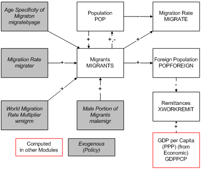

Although for most countries it is less important in determining population growth patterns than are fertility and mortality rate, migration is extremely important for some, such as those in the Arabian/Persian Gulf region. Because long-term migration is, however, very difficult to forecast, we rely on exogenous scenarios of migration rate (migrater ) to drive forecasts in IFs. Users can also affect global migration patterns with a multiplier on global rates (wmigrm ). On a global basis immigration and emigration are required to balance, and the number of migrants (MIGRANTS) in IFs is balanced, resulting in a computation also of an endogenous migration rate (MIGRATE).
Although data on age and sex of migrants are poor and certainly vary considerably by countries by origin and target, a general representation of the portion of migrants who are male (malemigr ) is set as a parameter. In addition, the migration rate by age is represented by an internal parameter set, migratebyage , read from a file and not available for users to change via the model interface. As rules of thumb, most migrants are male and disproportionately young adults.
The net of foreign-born population within a country relative to the size of a country’s diaspora abroad (POPFOREIGN) represents the accumulation of the net inflows of migrants over time. That population size and the level of GDP per capita determine the net extent of remittances sent or received from abroad.