Scenario Analysis
Scenario Description
A scenario is a story or story outline. Thinking about the future normally involves creating alternative scenarios, or stories, about the possible interactive evolution of variables. Some such scenarios are exploratory and consider the possible unfolding of different futures around key uncertainties, such as the rate of some aspect of technological advance or the fragility of some element in the global environment. Other scenarios are normative and develop stories about preferred futures, such as a global transformation to sustainability.
Scenarios in a computer model typically are built from multiple interventions that collectively help create a coherent story about the future. Often, but somewhat imprecisely, the word scenario is used more loosely to refer to any intervention (such as the change of a fertility rate for a country or an alternative assumption about oil resources).
Scenarios or interventions with respect to what? When IFs or other computer simulations are "run", without making any changes to parameters or initial conditions specified as the default values, they generate a forecast that is typically called the Base Case. The IFs Base Case, always available when a model session is initiated, is itself a scenario. Sometimes the Base Case is incorrectly referred to as a trend extrapolation or a "business as usual" scenario. More accurately, however, the IFs Base Case is a computation that involves the full dynamics of the model and therefore has very nonlinear behavior, often quite different from trends. It is a good starting point for scenario analysis for two reasons. First, it is built from initial conditions of all variables and on parameters that have been given reasonable values from data or other analysis. These initial conditions and parameters make up the package of interventions that constitute the Base Case scenario. Second, the Base Case is periodically analyzed relative to the forecasts of many other projects across the range of issue areas covered by IFs and is to a degree "tuned" for internal coherence and consistency with insights of respected forecasters.
There are two file types involved in IFs scenario creation: scenario files (or Scenario-Load-Files) and run files (or Run-Result-Files). Scenario files, the first type, are saved with an extension of .sce. Very small in size, .sce files contain information that the IFs model uses to create alternative scenarios; i.e., .sce files contain a list of parameter values that diverge from the Base Case. It is important to note that scenario files do not contain any forecasts. Forecasts are generated and saved only in the second type of file, run files with the .run extension. Because they contain forecasts of all IFs variables and parameters, .run files are much larger than scenario files. Although the IFs standalone model software allows users to save both types of files, web users are only able to save .sce files to retrieve their parameters and regenerate their scenarios.
In addition to the Base Case, most versions of IFs will include a number of other previously-run scenarios (see How Do I?/Lesson 0 for additional important terminology), typically those for the Global Environmental Outlook (GEO) of the United Nations Environmental Program (UNEP). If you look, for instance, at the Flexible Displays form, you will see a list of previously-run scenarios in the box at the bottom of the screen. Because those have already been run, based on a set of interventions constituting their foundations, the user can immediately display their results.
Quick Scenario Analysis with Tree Overview
Overview
What is a scenario?
This section of the help menu will guide you through a brief description of a scenario as well as the Base Case used in IFs and will discuss the difference between Scenario-Load-Files (.sce files) and Run-Result-Files (.run files).
After you have finished with this associated topic, you should be able to answer/do the following:
- What is a scenario?
- What is the Base Case of IFs?
- What is the difference between a Scenario-Load-File and a Run-Result-File?
Introduction to the Scenario Tree
The Quick Scenario Analysis with Tree allows you to call up or to mix and match an extensive number of your own interventions and/or a set of stored scenario intervention files. This feature of IFs allows you to change any parameter and selected initial conditions used in the model, thus shaping forecasts. Use the Quick Scenario Analysis with Tree to create Scenario-Load-Files and/or run scenario files through IFs in order to create Run-Result-Files that you can use throughout IFs.
Below is the main menu of the Quick Scenario Analysis with Tree:
Loading Previously-Structured Scenarios
The Quick Scenario Analysis with Tree allows you to load the previously-structured scenarios and user-saved scenarios. From the Scenario Files or the Adding Scenario Component menu options of the Quick Analysis with Tree, you can load a wide range of pre-packaged scenario intervention files and see what interventions were made in the files.
After you have finished with this topic, you should be able to do/answer the following:
- How does a previously-structured scenario differ from a previously-run scenario?
- What previously-structured scenarios came installed in your version of IFs?
- How does one search through the scenarios until you find one that deals with environmental change (or some other specific topic of interest)?
- What do you have to click on to understand exactly what is being changed by different previously-structured scenarios?
Finding the Intervention You Want
In order to tailor your scenario file to your needs, you must be able to quickly find the parameter you are looking for.
After you have finished with this topic, you should be able to do/answer the following:
- What is the organizational logic of the Scenario Tree?
- What is the difference between the Selected Initial Conditions, Relationship Parameters and the other five main categories used in the Scenario Tree?
- How would you search for a specific parameter that might help shape the scenario intervention of interest to you?
Exploring and Changing Parameters
Once you have found the parameter you are looking for, for instance, the total fertility rate multiplier (Households/Individuals, Demographic/Population, tfrm), a number of new options become available.
After you have finished with this topic, you should be able to do/answer the following:
- How do you select a parameter to change?
- What do the Select, Drivers, Explain, View Equations and Define pop-up options (when you click on a parameter name from the tree) all allow you to do?
- How do you clear parameter changes from the Scenario Tree?
- How do you create a Run-Result-File?
- How do you save the results?
- How can you display the results of your change in IFs?
Activate Pre-Run Scenario(s) for Display
Although not accessed through the scenario tree, it is important to know that hundreds of scenarios (the parameters for which are accessible in the tree) have been pre-run with the full forecasting results stored on the IFs server. It is not necessary for you to load the parameters and re-run these scenarios unless you want to create variations of them with new parameters or new parameter values. Instead you can go to the Display/Activate Pre-Run Scenario for Display sub-option of the Main Menu, choose the pre-run scenario, and then display results from it using any IFs display option.
Loading Previously-Structured Scenarios
Many packages of scenarios in IFs come pre-built. These previously-structured scenarios (that is, .sce files) are helpful components for building alternative futures in the model. They contain changes made in parameters but not yet in computed variables. They can be run to generate the forecasting results for all IFs variables (but if you are making no changes it will normally be easier simply to activate the results of running the .sce or scenario file). More often on the web-based version of IFs you will load an .sce file in order to make changes to it or to combine multiple .sce files.
There are two different ways of loading .sce files: the Add Scenario Component option (usually the easier of the two options) and the Open/Other sub-option under Scenario Files. Although the format of the two is different, the functionality is the same. From the main menu of Quick Scenario Analysis with Tree (reached with the Scenario Analysis option from the Main Menu of IFs), select Add Scenario Component and you will be presented with a drop-down list with the names of categories in which you can find different previously-structured scenarios, as shown below (the ultimate scenario names are often in sub-categories or even sub-sub categories because there are a large number of previously structured scenarios in IFs for your use). These scenarios can also be reached by clicking on the Scenario Files option (sub-option Open).
Any of the previously-structured scenarios can be loaded into the Scenario Tree of IFs. You can also create a larger scenario in the tree by adding several smaller scenarios together. Once you have loaded a scenario into the tree (experiment by doing so), if you would like to know more about the parameter changes from the Base Case that make up the scenario, click on Explain Scenario located on the menu.
Besides these previously-structured scenarios, hundreds of .sce files have been pre-run with the results saved as .run files (so called previously-run scenarios) on the web. Because previously-run files have already been run (as the name indicates) users can immediately display the results through different display options such as the Flexible Display and the Self-Managed Display. The menu that provides access to previously-run scenarios is the activate the results sub-option under Display from the Main Menu of IFs. By simply clicking the scenario name that the user would like to load, the activate feature would call it up. After activation, the user can see it in the scenario lists of the Flexible Display, for example. It is possible to activate multiple different scenarios by selecting them individually.
Parameter Types
Parameters are numbers that determine relationships among variables in the equations of IFs. You often set parameters to a single value across time and they therefore do not always "vary" as do "real" variables. Many parameters are "policy handles." More generally, parameters can actually be thought of as a special type of variable, the value of which you set in order to determine the behavior of the model. See the IFs project document called Guide to Scenario Analysis for much more information on parameter types and especially on the important parameters of IFs, organized by the models of the IFs system.
Multipliers: They have a normal value of 1, and to increase whatever they multiply (say agricultural yield) by 50 percent you increase the parameter to 1.5. To decrease it by 25 percent you would decrease the multiplier parameter to 0.75. You will almost always spread such changes out over time, keeping the multiplier's value at 1 in the base year and gradually increasing or decreasing it over a period of years. You should almost never change a multiplier in the initial year because the model is set up to provide accurate results for that year and will compensate for and thereby offset your change. For instance, if you set a multiplier on agricultural production equal to 1.5 for the first year and all years thereafter, you might find that the results were no different than in the base case. You must instead gradually introduce your change, preserving the multiplier value of "1" in the initial year. Examples of multipliers include: agdemm, enpm, freedomm, mortm, protecm, qem, rdm, resorm, tfrm, and ylm. Note that multipliers typically end with the letter "m".
Additive Factors: Most have a normal value of 0, thereby leaving that to which you add them unchanged. How much you would add to achieve a 50 percent increase might depend on the amount to which you added it to. Some additive parameters are, however, applied multiplicatively to the quantity they modify (that is, 1 plus the parameter is multiplied times the quantity), thereby scaling the parameter. In that case, the base or normal value of the parameter will be zero, but one can achieve a 50 percent increase in the quantity modified with a value of 0.5 and a 50 percent decrease with -0.5. You will very seldom want to change the base year value of additive parameters because it will either incorrectly change model results in the base year or, more likely, will result in model compensation to protect initial model results. An example of an additive parameter is: xshift (export shift as result of promotion of exports). Although early versions of IFs used additive factors and multipliers with comparable frequency, most additive factors have been replaced by multipliers to standardize most parameter changes.
Exponents: For instance, many "elasticities" raise something to a power. For these parameters the "normal value" will vary greatly, but they will most often fall between -2 and 2, with many clustering around 0. In most cases it will make sense to change these parameters for all years including the first - generally the model will not use them in the first year and they will affect results only in subsequent years. Elasticities in IFs include: elass and engel.
Reactivities: These are factors that relate growth in one process to growth in another. Although many will range between -2 and 2 (with 0 eliminating linkage of the processes), some have very large values. They are very much like elasticities, but the formulations that use them do not have exponential form. Reactivities include: cdmf, cpowdf, cwarf, nwarf, and reac.
Growth Rates: It is possible to force some processes to grow at specified rates. More commonly, the specified rates serve as targets and the dynamics of the model often shift actual growth rates somewhat, necessitating experimentation with targets to achieve a desired growth. Examples include: eprodr and tgrld.
Allocating Coefficients: Coefficients are often used in multiplicative relationships with other variables, but many such coefficients are not what were earlier called multipliers (with a base value of 1). Instead they can serve an allocating role. For instance, you can use parameters to allocate governmental spending to health, education, and the military. Allocating coefficients frequently have values between 0 and 1. Again, you should generally not change these parameters in the initial year because the model will often compensate for changed values in the first year. Instead, change them by series over time. Allocating coefficients in IFs include: aidlp, carabr, drcpow, drnpow, nmilf, and rfssh.
Transforming Coefficients: Some coefficients transform units of variables or link variables in other ways. Examples in IFs are: carfuel1, carfuel2, and carfuel3.
Switches: These parameters turn something on or off. They generally take on values of 1 (on) or 0 (off), but can have additional settings. For instance, some switches not only turn on some process, but set a key value within it (like the level of energy exports). Switches are most often on or off for the entire run, but it sometimes makes sense to "throw a switch" in the middle of a run. Switches allow you to fundamentally alter the structure of a model. Switches include: actreaon, agon, ally, enon, enprix, and squeez.
Variables: This category should technically not be called parameters at all. They could and would be computed endogenously, if the model included the appropriate theoretical structure. They generally do not determine the interaction of other variables. Such variables include: AQUACUL and EDPRIPTR.
Initial Conditions: Again, these are not strictly parameters, but rather first-year values for variables subsequently computed by the model. Although many initial conditions, like the population (POP) of the U.S., are sufficiently well-known that they should not be changed by model users, others, like the ultimate availability of oil and gas resources are only reasonable guesses. Thus users should feel free to change some initial conditions based on new data or even simply to test the implications. This category includes a great many variables, such as: AIDSDTHS and RESER.
The focus here is on exogenous parameters only - on those elements of the model that you can change. Many computed variables are used in the computation of other variables in the same way that parameters are, as multipliers, additive factors, coefficients, and so on. You can display those, but unlike true parameters, you cannot change them.
Finding Parameters and Variables
The main menu of Quick Scenario Analysis with Tree (found under Scenario Analysis from the Main Menu of IFs) provides you with a "tree" on the left hand side of the screen. This tree (Scenario Tree) represents all of the parameters and many of the initial conditions for variables used in IFs.
One way to find the parameter or variable initial condition you would like to change is to understand the general groupings of these categories (the main and secondary branches of the tree). The first two options or large branches on the tree, Technological Change and Environmental Uncertainties, lead you to primary parameters that allow you to shape the speed of technological change and the intensity of various environmental trends or constraints. The third, fourth and fifth main options on the tree, Households/Individuals, Governments/Social-Political Systems and Firms/Businesses, allow you to find and shape the primary parameters for the three main global actor categories. The Selected Initial Conditions option leads you to some of those for key IFs variables. Finally, the Relationship Parameters branch or option allows you to change all other model parameters in the model that are not identified in the branches above. Whereas most of the parameters accessed in the other branches are primary for scenario analysis, most of those opened by this branch more technically control model specifications and are unlikely to be altered by most users.
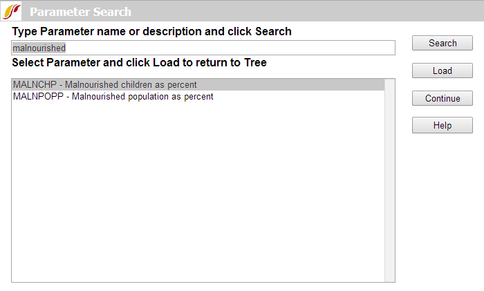
Another way for you to find the parameters you would like to change is by selecting the Parameter Search option near the right end of the form's menu. Clicking on this will bring up a window with a search box, as shown below. For example, if you are looking to work with the malnourished children parameters, type in "malnourished" and hit enter. This will bring up any parameter or variable initial condition with the word "malnourished" in its name or definition. You can also search for the parameter or variable by its name in IFs (like MALNCHP). If you know the parameter or initial condition you want to change (or its likely general characterization), it is often easier to search for it with this feature rather than by digging down into the branches of the tree.
From this window you can accomplish the following:
- Type Variable Name: In the top box, type in a variable name or a key word and click Search. This will bring up any variable/parameter that has your search term in its name/definition.
- Load: After you have located and clicked on a variable/parameter name you would like to manipulate in the tree, click Load. That will take you back to the Quick Scenario Analysis with Tree form and allow you to change values of it for scenario analysis.
- Continue: Click here if you would like to return to the scenario tree and its menu.
Clicking on and selecting a parameter or variable name for initial condition will bring up a small pop-up menu with the following three options to get more information about it: Define, Block Diagram and Equations.
Exploring and Changing Parameters
One of the key features of Quick Scenario Analysis with Tree is the ability to change specific variables and parameters.
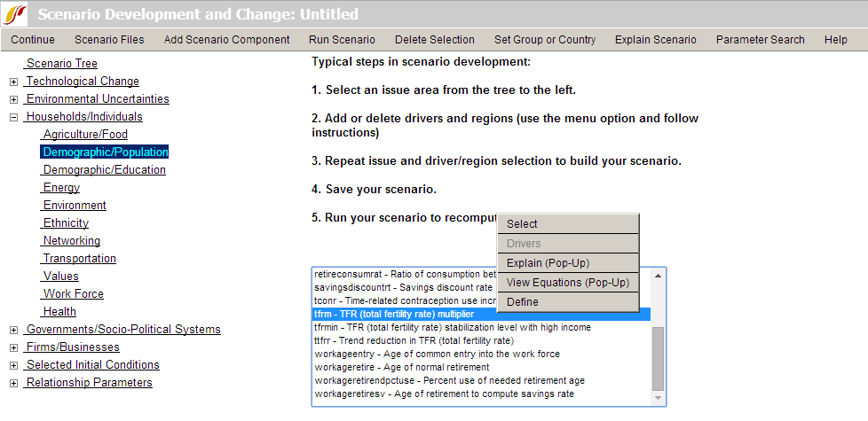
The image below shows you what becomes available to you if you click on a branch on the tree on the left side of the form, thereby generating the box of parameters accessible to you from that branch (see the box in the lower-right of the figure), and then click on the name of a specific parameter in the box (as with tfrm in the example). You are presented with five options in the pop-up: 1) Select the parameter in order to change it; 2) click on Drivers in order to see what variables are affecting what (may be de-activated); 3) click on Explain to see a causal diagram and an explanation of what this parameter affects; 4) click on View Equations to see the mathematical equations that link this parameter to variables; 5) click on Define to see a brief definition of what the parameter is and what it does.
In order to effectively use the Scenario Tree to change values, it is very useful to understand the different parameter types in the IFs system. See the Parameter Types topic. In the case of the tfrm parameter, it is a multiplier with a value of 1.0 in the Base Case. Because you selected a multiplier, the base-case value is always "1"—the model uses multipliers to easily raise or lower base-case values of many variables, and the multipliers are always "1" in the Base Case, so that values are unchanged by them. A multiplier can be distinguished from a variable because the ending of most multiplier abbreviations is the letter "m" such as tfrm.
You could use the Fully Customize option to create any pattern of intervention over time you desire, and at some point you should explore its use. But for now select the High option above the graph and note the change in the figure. This option will phase in a higher fertility (a 20% increase over the next ten years) for the country you select. Another type of simple change (short of full customization) is facilitated by the slider bar to the right of the graphic. Moreover, you can change the speed in which your increase or decrease in tfrm takes place with the drop-down list labeled "Shift Years:" above the graph. Again, if you would like more control over your parameters, you can click on the Fully Customize button located below the graph and you will be presented with a new form.
If you have mistakenly changed a parameter and you would like to remove your alteration, simply click on the parameter change you would like to remove and then click on the Delete Selection option (sub-option Delete) from the menu. If you would like to clear all the changes made to the Scenario Tree, simply click on the Clear Tree sub-option located under Scenario Files.
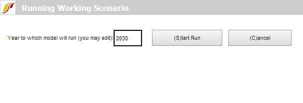
If you have changed a parameter, it will affect nothing else until you run the model and recalculate all of the variables in it for all of the countries. That is, if you have created a Scenario-Load-File (.sce) in order to analyze your scenario, you need a Run-Result-File (.run). Click on the Run Scenario option then the Run sub-option from the menu. Your parameter will first be loaded into the working file. You will then be shown the Running Working Scenario form. You can change the end year or leave it as is. Click on Start Run for IFs to create a new run-file based on your specifications.
After IFs has recomputed the model with your new parameter(s) and temporarily saved the results as a .run file, you will be presented with a screen that says, "Run Successful – Click to Continue." The resulting Working File (temporarily saved .run file) with new forecast computations will now be available for your analysis by itself or in comparison with the Base Case or other scenarios. Look, for instance, at Gross Domestic Product (GDP) and GDP per capita (GDPPC) of your country before and after the intervention by selecting both 0-Working File and 1-IFSBASE.run (IFs Base Case) in the Flexible Displays. If the country or grouping for which you changed one or more parameters was fairly large, you will see changes in many variables elsewhere around the world. Note that when you exit from IFs, the revised Working File will be lost. In order to get it again, you will need to go to the Scenario Tree, retrieve your scenario file, and run it again.
In order to hold onto parameter changes you make and a scenario you may want to explore again or develop further, return to Quick Scenario Analysis with Tree and select the Scenario Files option, Name and Save sub-option. Give your scenario file and folder names. The parameter intervention in the form of a .sce file (but not the full results after your run) can be saved in the system for one month and can be retrieved under Add Scenario Component/User Defined Scenarios/your folder, or under Scenario Files/Open/Other/User Defined Scenarios/your folder. If you would like to keep your intervention permanently, click on the Export Working File sub-option under Scenario Files. You will be asked to choose where you would like to save your scenario and under what name. This will allow you to save your scenario file (.sce file) on your hard drive. Although you will not be able to bring this file saved in your machine back to the web-version of IFs, it is possible to use the .sce file with the stand-alone version of IFs; it is best if your file is stored in the Scenario folder under IFs on your hard drive (C:/Users/Public/IFs/Scenario).
Customization of Parameters
The Exploring and Changing Parameters Topic explains the general use of the Scenario Tree to identify and begin to change parameters. The Fully Customize option calls up a specialized form that allows greater control over changes than the High/Low/Base radio buttons or the slider bar on the scenario tree form itself.
Alternative Ways to Use the Change Values Form:
- Specify a Desired Value for One or More Years. You specify a desired numerical value, indicate the number of years you wish to repeat that value (one or more) and then touch the Change/Repeat button.
- Interpolate to a Desired Value over Several Years. You specify a desired value, indicate the number of years over which you wish to interpolate to that value, and then touch the Interpolate button.
- Cancel All Changes (only becomes active after you have made changes). You touch the Cancel All Changes button to revert to the parameter values before you began making changes.
- Move Forward or Backward Across Years. You touch the Previous Year or the Next Year buttons to move across time without changing parameter values.
The graphic in the upper right of the form will show you the changes made. You can also use the slider bar below that graphic to make changes.
When changes are complete, Exit to Scenario Tree will take you back to the tree.
Change Selected Functions
Variables are forecast based on mathematic relationships that are represented by functions within IFs. These functions can be changed by users based on different understandings of relationships between variables. Users of IFs can change relationships between two variables or multiple variables . Follow the links below to learn more about how to change these relationships.
Bivariate Functions
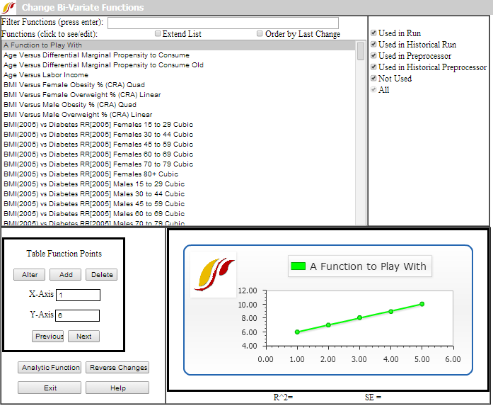
Begin at the Main Menu of IFs. Choose the Change Selected Functions option under Scenario Analysis. Then choose the Bivariate Functions sub-option. That will give you the Change Bi-Variate Functions window, below.
To see the full list of functions or relationships that you can change in IFs, check Extend List. Click on any of the function names (relationships) in the Functions list box in order to see the relationship already in IFs. When you click a graphic of the function will be displayed in the lower right of the window. Many of the functions will also display the r-squared and standard error (SE) that indicate the strength of the relationship that we found when creating it via cross-sectional analysis of our database.
Our creation of the functions was sometimes to use in computations of the model run from the base year, sometimes to be used in the historical run, and sometimes in the model's data preprocessor to fill holes and clean up data (again, for either historical forecasts or those looking forward). The options in the upper right are all checked by default, but if you wanted to see only those functions used in the model run, you could turn off all of the other checks. This window actually gives you the opportunity to revise the functions used in the model run.
There are two ways to specify (and therefore also to change) relationships in IFs. The first is called a "table function." Table functions allow you to specify two or more points in a relationship and let IFs connect those points with lines to create the relationship. This is a very simple process because you need not understand equations; but it also allows the creation of complex functions. The second is via "analytic functions" or equations. Look at each in turn.
Option A for Specifying Relationships: Table Functions. Click on the "A Function to Play With" relationship so that you can do just that. In the Table Function Points frame, you see boxes for specifying new or changing old X-axis and Y-axis values. Let's start by adding a point to the five that already make up the table function. Specify 7 as the X-axis value and 8 as the Y-axis value. Touch the Add button and the point will be added, creating a relationship between X and Y that increases to a point and then starts down. Try specifying 1 as the X-axis value and 8 as the Y-axis value, then touching the Alter button. Now you have a relationship that starts downward, climbs, and then drops. Table functions give you nearly unlimited control over the form of a relationship. You can always touch Reverse Changes to return to the original form. As it says, play around.
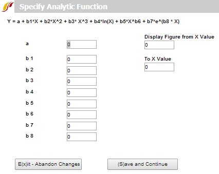
Option B for Specifying Relationships: Analytic Functions (Equations). Click again on the "A Function to Play With" relationship. This time, however, touch the Analytic Function button in the lower left to call up the following screen.
If you do not understand equations, you may want to skip this part of the lesson – table functions can serve you well. But you can create a simple analytical function by specifying the constant (a) as 20 and the logarithmic parameter (b4) as 3. Leave the other parameters at 0. Note that by selectively specifying various parameters you can create a wide variety of analytic functions (including most of those that Excel will create when you fit lines to scatter plots). You may also specify the lower and upper range over which you will allow the independent variable to vary. For instance, you may not want the independent variable to be negative.
Save and Continue returns you to the Change Functions window and displays the analytic form you have specified. Note that the function you have created looks much like the one that Excel fit to the relationship between GDP per capita and life expectancy in Lesson 4 . You now have the capability of discovering relationships and good analytic representations of them using the cross-section analysis capability of IFs or Excel with the IFs database or Excel and then taking those relationships into IFs itself.
When you Exit from the Change Functions window, IFs gives you a very important informational warning. If you have made any changes to functions, those will remain active only until you exit from IFs. Starting IFs again resets all functions to standard values. Moreover, although runs of the model that you make with altered functions will reflect your changes, no information about the changed functions is saved with the .RUN files. You must keep track of the changes you make in functions.
After you have changed one or more functions, you can run the model and create a new working file that reflects the changed functions and their impact on all computations in IFs. You can compare that working file (or a saved version of it) with the Base Case or with other scenarios.
Multivariate Functions
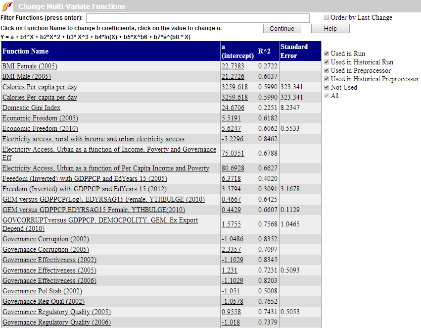
Begin at the Main Menu of IFs. Choose the Change Selected Functions option under Scenario Analysis. Then choose the Multivariate Functions sub-option. That will give you the Change Multi-Variate Functions window, below.
Our creation of the functions was most often to use in computations of the model run from the base year, sometimes to be used in the historical run, and sometimes in the model's data preprocessor to fill holes and clean up data (again, for either historical forecasts or those looking forward). The options in the upper right are all checked by default, but if you wanted to see only those functions used in the model run, you could turn off all of the other checks. This form actually gives you the opportunity to revise the functions used in the model run.
The form has two grids. The first grid on the default page shows a list of all multivariate functions in the model. When you select one of the functions in the first grid, the second grid will show up, which shows the independent variables and parameters in the particular function you have chosen.
- Intercepts: Change the intercept value for the function by left-clicking on the value in the intercept cell of the function of interest (the intercept cell is just to the right of the name of the dependent variable).
- Other Parameters: Change parameters associated with specific independent variables for a selected function by clicking on the appropriate cell and changing values as desired. The general function at the top of the form explains the meaning of each possible parameter for independent variables. For instance, b1 is the parameter and would be used to identify a linear relationship of the independent and dependent variables. Normally, of course, most parameters will be zero (or null which means 0).
Changing functions gives you a powerful tool for using IFs to investigate possible futures. To an extent, it allows you to change the model itself.
Running Working Scenario
The Run option can be found by selecting Scenario Analysis from the Main Menu.
Use this IFs option if you would like to take a Working File to which you have made scenario changes (see the topic on Quick Scenario Analysis with Tree) and run it so that all of the variables of IFs are recomputed. It is important to remember that scenario changes of parameters or initial conditions by themselves do not affect the forecasted variables of IFs. It requires a run of the model to do those computations. When the run is completed after parameter changes, the forecast variables of the Working File will have been completely changed.
Entering this form directly from the Main Menu is actually not the most common path. Typically, users will change parameters in the Quick Scenario Tree and use the Run option from that form. It will also take them to this form for Running (the) Working Scenario.
On this form you can specify for how many years IFs should run. Choose the year in which you would like the run to stop and then click Start Run.
Reload the Base
When you have used the scenario tree (see Quick Analysis with Scenario Tree) to build a scenario via parameter changes or to load a pre-existing set of parameter changes (an .sce file) and then run the scenario to generate a run or results file, the Working File will hold the contents of that model run. It will therefore be different from the Base Case, to which it is automatically set every time you start IFs again. Should you wish to reset the Working File to the Base Case in a session of work with IFs, simply use the Reload the Base sub-option under the Scenario Analysis option of the Main Menu.


