SubRegionalization Handbook: Difference between revisions
AltheaDitter (talk | contribs) No edit summary |
MeredithMoon (talk | contribs) No edit summary |
||
| (15 intermediate revisions by one other user not shown) | |||
| Line 1: | Line 1: | ||
= Foundational Elements = | = Foundational Elements = | ||
= A Note on Terminology = | == A Note on Terminology == | ||
Sub-regional units go by many names internationally. When we refer to a sub-region in this document, we may use a variety of names to refer to the same entity. In IFs, there is a bias toward the use of “province” to refer to a sub-regional unit, but it is functionally equivalent to states, departments, territories, or any other name for a sub-regional unit. | Sub-regional units go by many names internationally. When we refer to a sub-region in this document, we may use a variety of names to refer to the same entity. In IFs, there is a bias toward the use of “province” to refer to a sub-regional unit, but it is functionally equivalent to states, departments, territories, or any other name for a sub-regional unit. | ||
| Line 11: | Line 11: | ||
=== IFsHistSeriesXXX.mdb === | === IFsHistSeriesXXX.mdb === | ||
Before a country in IFs can be divided into | Before a country in IFs can be divided into sub-regions, a new data file called ''IFsHistSeriesXXX.mdb,'' for example ''IFsHistSeriesChina.mdb,'' must be created. That file is a variation of the file called ''IFsHistSeries.mdb'', which contains data tables for all countries across time, for all variables. | ||
For each data table in ''IFsHistSeriesXXX.mdb'', rows correspond to all states/provinces/departments in the specified country. The file includes a table called ''DataDict ''which is analogous to the file ''DataDict.mdb ''and provides information on names, sources, and specialized procedures followed to prepare the state/province/department data. | For each data table in ''IFsHistSeriesXXX.mdb'', rows correspond to all states/provinces/departments in the specified country. The file includes a table called ''DataDict ''which is analogous to the file ''DataDict.mdb ''and provides information on names, sources, and specialized procedures followed to prepare the state/province/department data. | ||
| Line 20: | Line 20: | ||
*Select the country that is intended to be subregionalized and click ''OK'' | *Select the country that is intended to be subregionalized and click ''OK'' | ||
This does a couple things. First, it creates a new ''IFsHistSeries.mdb'' for the country you selected in ''C:\Users\Public\IFs\DATA''. The file will include tables for the 4 essential series and a datadict. It also adds the country to the ''Provinces'' tables in ''Provinces.mdb''. | This does a couple of things. First, it creates a new ''IFsHistSeries.mdb'' for the country you selected in ''C:\Users\Public\IFs\DATA''. The file will include tables for the 4 essential series and a datadict. It also adds the country to the ''Provinces'' tables in ''Provinces.mdb''. | ||
The entire process of sub-regionalization affects five files:''IFs.mdb, IFsHistSeries.mdb, IFsCoVatra.mdb, IFsCoVatraSeries.mdb,''and ''IFsWVSCohort.mdb''. For each of the files, the process looks in the ''IFs\Data'' folder for an equivalent file with the name of the country at the end — again, ''IFsHistSeriesChina.mdb'' is an example — then creates a copy in the''IFs\Runfiles'' directory. Modification is done in the copies on the ''\Runfiles ''directory as well to the original files in the ''\Data'' directory. Data for individual sub-regional units and the country as a whole are preserved, and can be copied back and forth between ''\Data'' and ''\Runfiles'' directories. This allows the user to switch between model runs with different sub-regionalizations, and reset everything to the starting point without any states/provinces/departments sub-regionalized. | The entire process of sub-regionalization affects five files:''IFs.mdb, IFsHistSeries.mdb, IFsCoVatra.mdb, IFsCoVatraSeries.mdb,''and ''IFsWVSCohort.mdb''. For each of the files, the process looks in the ''IFs\Data'' folder for an equivalent file with the name of the country at the end — again, ''IFsHistSeriesChina.mdb'' is an example — then creates a copy in the''IFs\Runfiles'' directory. Modification is done in the copies on the ''\Runfiles ''directory as well to the original files in the ''\Data'' directory. Data for individual sub-regional units and the country as a whole are preserved, and can be copied back and forth between ''\Data'' and ''\Runfiles'' directories. This allows the user to switch between model runs with different sub-regionalizations, and reset everything to the starting point without any states/provinces/departments sub-regionalized. | ||
| Line 38: | Line 38: | ||
In addition to the creation of ''IFsHistSeriesXXX.mdb'', initiating the sub-regionalization process requires modifications to tables that exist in the file ''Provinces.mdb''. The alterations to specific tables in ''Provinces.mdb'' are outlined below: | In addition to the creation of ''IFsHistSeriesXXX.mdb'', initiating the sub-regionalization process requires modifications to tables that exist in the file ''Provinces.mdb''. The alterations to specific tables in ''Provinces.mdb'' are outlined below: | ||
'''All Provinces'''. The name and FIPS code of the target country should be added to a line in this table (those names should be identical to those used for the country in ''IFs.mdb'' and ''IFsHistSeries.mdb'' files; and province break-out should only be done when the Full version of IFs is being used with each country represented as a separate region). The ''AllProvinces'' field should | '''All Provinces'''. The name and FIPS code of the target country should be added to a line in this table (those names should be identical to those used for the country in ''IFs.mdb'' and ''IFsHistSeries.mdb'' files; and province break-out should only be done when the Full version of IFs is being used with each country represented as a separate region). The ''AllProvinces'' field should be checked. The only circumstances under which it is not checked is when the user is selecting one, or a few, provinces for use in the model in addition to the entire country — see the discussion of the ''Regionalization'' table below. | ||
'''Provinces'''. In this table all of the provinces or states should be identified. The first column is the target country (the same for all provinces). The second is a unique FIPS Code created by the user (since country-specific codes are three letters and cannot be duplicated, two-letter codes normally work well for these). Finally, the name of the sub-regional unit should be specified. | '''Provinces'''. In this table all of the provinces or states should be identified. The first column is the target country (the same for all provinces). The second is a unique FIPS Code created by the user (since country-specific codes are three letters and cannot be duplicated, two-letter codes normally work well for these). Finally, the name of the sub-regional unit should be specified. | ||
| Line 50: | Line 50: | ||
'''Regionalization'''. This table repeats the target ''Country'' and ''Full Province Name'' as in the ''Provinces'' table. The new feature is the addition of a ''Region'' name. Each province could be a separate ''Region'', in which case the names should be less than 10-12 letters so as to allow easy display in IFs tables and graphs. Most often the provinces will be grouped into sub-regions of the target Country, in which case it is recommended that the ''Region'' name be the target country name or some abbreviated part of it followed by the sub-region, again a total of no more than 10-12 letters. Leading with the Country name facilitates the use of alphabetic listings of IFs. | '''Regionalization'''. This table repeats the target ''Country'' and ''Full Province Name'' as in the ''Provinces'' table. The new feature is the addition of a ''Region'' name. Each province could be a separate ''Region'', in which case the names should be less than 10-12 letters so as to allow easy display in IFs tables and graphs. Most often the provinces will be grouped into sub-regions of the target Country, in which case it is recommended that the ''Region'' name be the target country name or some abbreviated part of it followed by the sub-region, again a total of no more than 10-12 letters. Leading with the Country name facilitates the use of alphabetic listings of IFs. | ||
If the user is only adding a single province (or a very small number) to the model and not splitting a country into regions based on all states/provinces, the lines added to the ''Regionalization'' table will be only for the added states/provinces (e.g. Hawaii could be added in addition to the US by adding a line to this table for it only, not other US states, and then not checking AllProvinces in the AllProvinces table). Even if all provinces/states are in the data set, as with India, this process allows a single state of India to be pulled out and added to IFs. '''Warning''': if a user only adds | If the user is only adding a single province (or a very small number) to the model and not splitting a country into regions based on all states/provinces, the lines added to the ''Regionalization'' table will be only for the added states/provinces (e.g. Hawaii could be added in addition to the US by adding a line to this table for it only, not other US states, and then not checking AllProvinces in the AllProvinces table). Even if all provinces/states are in the data set, as with India, this process allows a single state of India to be pulled out and added to IFs. | ||
'''Warning''': if a user only adds sub-regions rather than dividing a country into sub-regions based on all of them, there will be double counting of the country and the added unit(s) in the model. Only selected variables in IFs, such as ''WPOP'' and variables of the agricultural model have been set up for correction of such double counting in the run of the model. | |||
The process of creation of regions can be done within IFs, under: | The process of creation of regions can be done within IFs, under: | ||
| Line 291: | Line 293: | ||
Select ''OK'' to this message and then click ''Run Successful – Click to Continue''. | Select ''OK'' to this message and then click ''Run Successful – Click to Continue''. | ||
=== Switching Models === | |||
It is also possible to switch between different model runs (i.e. between the national level and a sub-regional model). For instance, you have just completed a sub-regionalization that divides China into single provinces. Now, you would like to use data for the whole country as a Base Case again. To remove all sub-regions, open the window for ''Add or Delete Subregions''. Click on ''Switch Provinces'' and choose ''No State/Province'' from the right side box of Available Runs. Click ''Switch'' to restore the model to pre-sub-regionalization status. | It is also possible to switch between different model runs (i.e. between the national level and a sub-regional model). For instance, you have just completed a sub-regionalization that divides China into single provinces. Now, you would like to use data for the whole country as a Base Case again. To remove all sub-regions, open the window for ''Add or Delete Subregions''. Click on ''Switch Provinces'' and choose ''No State/Province'' from the right side box of Available Runs. Click ''Switch'' to restore the model to pre-sub-regionalization status. | ||
At this point you will be asked if you want to save your current configuration. It is important to select ''Yes'' in order switch back to the preferred sub-regionalization the next time you want to revert back to the sub-regional version. | At this point you will be asked if you want to save your current configuration. It is important to select ''Yes'' in order switch back to the preferred sub-regionalization the next time you want to revert back to the sub-regional version. This process only takes 5 - 10 minutes, so it is possible to switch back and forth on a regular basis. | ||
==== Switching Models to Process New Data ==== | |||
To process newly imported data for the preferred sub-regionalization, the existing sub-region setup (used for switching) needs to be removed first and the model needs to be broken out again. To do this users must switch their model from the broken out version to the ''No State/Province'' version as described above. The option to delete a sub-region setup is in the same window as to add sub-regions. After the model has been switched to No State/Province select the country from the box on the right, ''Available Runs:'' and click ''Remove ''to delete the sub-region setup. Deleting a sub-region setup will remove all files created in the process of adding the sub-region setup, and the corresponding model run will no longer be available from the Switch Provinces option. | |||
= Appendix = | = Appendix = | ||
| Line 1,606: | Line 1,592: | ||
Instead of taking the average as was done for females, the model uses a weighted average based on GDP data. In other words, each life expectancy value is multiplied by the state’s proportional GDP contribution to the total GDP for all states, then the resulting values are summed. | Instead of taking the average as was done for females, the model uses a weighted average based on GDP data. In other words, each life expectancy value is multiplied by the state’s proportional GDP contribution to the total GDP for all states, then the resulting values are summed. | ||
{| border="1" cellspacing="0" cellpadding="0" width="574" style="width:573px;" | |||
|- | |||
| nowrap="nowrap" style="width:161px;height:17px;" | | |||
SeriesLifExpectMale | |||
| nowrap="nowrap" style="width:65px;height:17px;" | | |||
| |||
| nowrap="nowrap" style="width:217px;height:17px;" | | |||
| |||
| nowrap="nowrap" style="width:130px;height:17px;" | | |||
| |||
|- | |||
| nowrap="nowrap" style="width:161px;height:17px;" | | |||
Country | |||
| nowrap="nowrap" style="width:65px;height:17px;" | | |||
MostRecent | |||
| nowrap="nowrap" style="width:217px;height:17px;" | | |||
Weights (State GDP/Total GDP for States) | |||
| nowrap="nowrap" style="width:130px;height:17px;" | | |||
(MostRecent)*(Weights) | |||
|- | |||
| nowrap="nowrap" style="width:161px;height:17px;" | | |||
Andaman and Nicobar Islands | |||
| nowrap="nowrap" style="width:65px;height:17px;" | | |||
<span style="background-color:#FF8C00;">63.62</span> | |||
| nowrap="nowrap" style="width:217px;height:17px;" | | |||
0.001 | |||
| nowrap="nowrap" style="width:130px;height:17px;" | | |||
0.04 | |||
|- | |||
| nowrap="nowrap" style="width:161px;height:17px;" | | |||
Andhra Pradesh | |||
| nowrap="nowrap" style="width:65px;height:17px;" | | |||
66.90 | |||
| nowrap="nowrap" style="width:217px;height:17px;" | | |||
0.081 | |||
| nowrap="nowrap" style="width:130px;height:17px;" | | |||
5.42 | |||
|- | |||
| nowrap="nowrap" style="width:161px;height:17px;" | | |||
Arunachal Pradesh | |||
| nowrap="nowrap" style="width:65px;height:17px;" | | |||
<span style="background-color:#FF8C00;">63.62</span> | |||
| nowrap="nowrap" style="width:217px;height:17px;" | | |||
0.001 | |||
| nowrap="nowrap" style="width:130px;height:17px;" | | |||
0.08 | |||
|- | |||
| nowrap="nowrap" style="width:161px;height:17px;" | | |||
Assam | |||
| nowrap="nowrap" style="width:65px;height:17px;" | | |||
63.60 | |||
| nowrap="nowrap" style="width:217px;height:17px;" | | |||
0.016 | |||
| nowrap="nowrap" style="width:130px;height:17px;" | | |||
0.99 | |||
|- | |||
| nowrap="nowrap" style="width:161px;height:17px;" | | |||
Bihar | |||
| nowrap="nowrap" style="width:65px;height:17px;" | | |||
68.60 | |||
| nowrap="nowrap" style="width:217px;height:17px;" | | |||
0.028 | |||
| nowrap="nowrap" style="width:130px;height:17px;" | | |||
1.94 | |||
|- | |||
| nowrap="nowrap" style="width:161px;height:17px;" | | |||
Chandigarh | |||
| nowrap="nowrap" style="width:65px;height:17px;" | | |||
<span style="background-color:#FF8C00;">63.62</span> | |||
| nowrap="nowrap" style="width:217px;height:17px;" | | |||
0.003 | |||
| nowrap="nowrap" style="width:130px;height:17px;" | | |||
0.18 | |||
|- | |||
| nowrap="nowrap" style="width:161px;height:17px;" | | |||
Chhatisgarh | |||
| nowrap="nowrap" style="width:65px;height:17px;" | | |||
<span style="background-color:#FF8C00;">63.62</span> | |||
| nowrap="nowrap" style="width:217px;height:17px;" | | |||
0.017 | |||
| nowrap="nowrap" style="width:130px;height:17px;" | | |||
1.05 | |||
|- | |||
| nowrap="nowrap" style="width:161px;height:17px;" | | |||
Dadra and Nagar Haveli | |||
| nowrap="nowrap" style="width:65px;height:17px;" | | |||
<span style="background-color:#FF8C00;">63.62</span> | |||
| nowrap="nowrap" style="width:217px;height:17px;" | | |||
0.000 | |||
| nowrap="nowrap" style="width:130px;height:17px;" | | |||
0.02 | |||
|- | |||
| nowrap="nowrap" style="width:161px;height:17px;" | | |||
Daman and Diu | |||
| nowrap="nowrap" style="width:65px;height:17px;" | | |||
<span style="background-color:#FF8C00;">63.62</span> | |||
| nowrap="nowrap" style="width:217px;height:17px;" | | |||
0.000 | |||
| nowrap="nowrap" style="width:130px;height:17px;" | | |||
0.01 | |||
|- | |||
| nowrap="nowrap" style="width:161px;height:17px;" | | |||
Delhi | |||
| nowrap="nowrap" style="width:65px;height:17px;" | | |||
<span style="background-color:#FF8C00;">63.62</span> | |||
| nowrap="nowrap" style="width:217px;height:17px;" | | |||
0.035 | |||
| nowrap="nowrap" style="width:130px;height:17px;" | | |||
2.23 | |||
|- | |||
| nowrap="nowrap" style="width:161px;height:17px;" | | |||
Goa | |||
| nowrap="nowrap" style="width:65px;height:17px;" | | |||
<span style="background-color:#FF8C00;">63.62</span> | |||
| nowrap="nowrap" style="width:217px;height:17px;" | | |||
0.005 | |||
| nowrap="nowrap" style="width:130px;height:17px;" | | |||
0.30 | |||
|- | |||
| nowrap="nowrap" style="width:161px;height:17px;" | | |||
Gujarat | |||
| nowrap="nowrap" style="width:65px;height:17px;" | | |||
69.20 | |||
| nowrap="nowrap" style="width:217px;height:17px;" | | |||
0.072 | |||
| nowrap="nowrap" style="width:130px;height:17px;" | | |||
5.00 | |||
|- | |||
| nowrap="nowrap" style="width:161px;height:17px;" | | |||
Haryana | |||
| nowrap="nowrap" style="width:65px;height:17px;" | | |||
66.50 | |||
| nowrap="nowrap" style="width:217px;height:17px;" | | |||
0.036 | |||
| nowrap="nowrap" style="width:130px;height:17px;" | | |||
2.40 | |||
|- | |||
| nowrap="nowrap" style="width:161px;height:17px;" | | |||
Himachal Pradesh | |||
| nowrap="nowrap" style="width:65px;height:17px;" | | |||
68.90 | |||
| nowrap="nowrap" style="width:217px;height:17px;" | | |||
0.008 | |||
| nowrap="nowrap" style="width:130px;height:17px;" | | |||
0.55 | |||
|- | |||
| nowrap="nowrap" style="width:161px;height:17px;" | | |||
Jammu & Kashmir | |||
| nowrap="nowrap" style="width:65px;height:17px;" | | |||
<span style="background-color:#FF8C00;">63.62</span> | |||
| nowrap="nowrap" style="width:217px;height:17px;" | | |||
0.008 | |||
| nowrap="nowrap" style="width:130px;height:17px;" | | |||
0.51 | |||
|- | |||
| nowrap="nowrap" style="width:161px;height:17px;" | | |||
Jharkhand | |||
| nowrap="nowrap" style="width:65px;height:17px;" | | |||
<span style="background-color:#FF8C00;">63.62</span> | |||
| nowrap="nowrap" style="width:217px;height:17px;" | | |||
0.018 | |||
| nowrap="nowrap" style="width:130px;height:17px;" | | |||
1.12 | |||
|- | |||
| nowrap="nowrap" style="width:161px;height:17px;" | | |||
Karnataka | |||
| nowrap="nowrap" style="width:65px;height:17px;" | | |||
68.00 | |||
| nowrap="nowrap" style="width:217px;height:17px;" | | |||
0.057 | |||
| nowrap="nowrap" style="width:130px;height:17px;" | | |||
3.87 | |||
|- | |||
| nowrap="nowrap" style="width:161px;height:17px;" | | |||
Kerala | |||
| nowrap="nowrap" style="width:65px;height:17px;" | | |||
73.20 | |||
| nowrap="nowrap" style="width:217px;height:17px;" | | |||
0.037 | |||
| nowrap="nowrap" style="width:130px;height:17px;" | | |||
2.68 | |||
|- | |||
| nowrap="nowrap" style="width:161px;height:17px;" | | |||
Lakshadweep | |||
| nowrap="nowrap" style="width:65px;height:17px;" | | |||
<span style="background-color:#FF8C00;">63.62</span> | |||
| nowrap="nowrap" style="width:217px;height:17px;" | | |||
0.000 | |||
| nowrap="nowrap" style="width:130px;height:17px;" | | |||
0.01 | |||
|- | |||
| nowrap="nowrap" style="width:161px;height:17px;" | | |||
Madhya Pradesh | |||
| nowrap="nowrap" style="width:65px;height:17px;" | | |||
57.00 | |||
| nowrap="nowrap" style="width:217px;height:17px;" | | |||
0.037 | |||
| nowrap="nowrap" style="width:130px;height:17px;" | | |||
2.08 | |||
|- | |||
| nowrap="nowrap" style="width:161px;height:17px;" | | |||
Maharashtra | |||
| nowrap="nowrap" style="width:65px;height:17px;" | | |||
64.50 | |||
| nowrap="nowrap" style="width:217px;height:17px;" | | |||
0.144 | |||
| nowrap="nowrap" style="width:130px;height:17px;" | | |||
9.26 | |||
|- | |||
| nowrap="nowrap" style="width:161px;height:17px;" | | |||
Manipur | |||
| nowrap="nowrap" style="width:65px;height:17px;" | | |||
<span style="background-color:#FF8C00;">63.62</span> | |||
| nowrap="nowrap" style="width:217px;height:17px;" | | |||
0.001 | |||
| nowrap="nowrap" style="width:130px;height:17px;" | | |||
0.08 | |||
|- | |||
| nowrap="nowrap" style="width:161px;height:17px;" | | |||
Meghalaya | |||
| nowrap="nowrap" style="width:65px;height:17px;" | | |||
68.90 | |||
| nowrap="nowrap" style="width:217px;height:17px;" | | |||
0.002 | |||
| nowrap="nowrap" style="width:130px;height:17px;" | | |||
0.14 | |||
|- | |||
| nowrap="nowrap" style="width:161px;height:17px;" | | |||
Mizoram | |||
| nowrap="nowrap" style="width:65px;height:17px;" | | |||
<span style="background-color:#FF8C00;">63.62</span> | |||
| nowrap="nowrap" style="width:217px;height:17px;" | | |||
0.001 | |||
| nowrap="nowrap" style="width:130px;height:17px;" | | |||
0.06 | |||
|- | |||
| nowrap="nowrap" style="width:161px;height:17px;" | | |||
Nagaland | |||
| nowrap="nowrap" style="width:65px;height:17px;" | | |||
<span style="background-color:#FF8C00;">63.62</span> | |||
| nowrap="nowrap" style="width:217px;height:17px;" | | |||
0.002 | |||
| nowrap="nowrap" style="width:130px;height:17px;" | | |||
0.10 | |||
|- | |||
| nowrap="nowrap" style="width:161px;height:17px;" | | |||
Orissa | |||
| nowrap="nowrap" style="width:65px;height:17px;" | | |||
64.30 | |||
| nowrap="nowrap" style="width:217px;height:17px;" | | |||
0.027 | |||
| nowrap="nowrap" style="width:130px;height:17px;" | | |||
1.76 | |||
|- | |||
| nowrap="nowrap" style="width:161px;height:17px;" | | |||
Pondicherry | |||
| nowrap="nowrap" style="width:65px;height:17px;" | | |||
69.70 | |||
| nowrap="nowrap" style="width:217px;height:17px;" | | |||
0.002 | |||
| nowrap="nowrap" style="width:130px;height:17px;" | | |||
0.13 | |||
|- | |||
| nowrap="nowrap" style="width:161px;height:17px;" | | |||
Punjab | |||
| nowrap="nowrap" style="width:65px;height:17px;" | | |||
67.40 | |||
| nowrap="nowrap" style="width:217px;height:17px;" | | |||
0.031 | |||
| nowrap="nowrap" style="width:130px;height:17px;" | | |||
2.11 | |||
|- | |||
| nowrap="nowrap" style="width:161px;height:17px;" | | |||
Rajasthan | |||
| nowrap="nowrap" style="width:65px;height:17px;" | | |||
67.60 | |||
| nowrap="nowrap" style="width:217px;height:17px;" | | |||
0.047 | |||
| nowrap="nowrap" style="width:130px;height:17px;" | | |||
3.17 | |||
|- | |||
| nowrap="nowrap" style="width:161px;height:17px;" | | |||
Sikkim | |||
| nowrap="nowrap" style="width:65px;height:17px;" | | |||
<span style="background-color:#FF8C00;">63.62</span> | |||
| nowrap="nowrap" style="width:217px;height:17px;" | | |||
0.001 | |||
| nowrap="nowrap" style="width:130px;height:17px;" | | |||
0.07 | |||
|- | |||
| nowrap="nowrap" style="width:161px;height:17px;" | | |||
Tamil Nadu | |||
| nowrap="nowrap" style="width:65px;height:17px;" | | |||
64.20 | |||
| nowrap="nowrap" style="width:217px;height:17px;" | | |||
0.081 | |||
| nowrap="nowrap" style="width:130px;height:17px;" | | |||
5.21 | |||
|- | |||
| nowrap="nowrap" style="width:161px;height:17px;" | | |||
Telangana | |||
| nowrap="nowrap" style="width:65px;height:17px;" | | |||
68.60 | |||
| nowrap="nowrap" style="width:217px;height:17px;" | | |||
0.041 | |||
| nowrap="nowrap" style="width:130px;height:17px;" | | |||
2.81 | |||
|- | |||
| nowrap="nowrap" style="width:161px;height:17px;" | | |||
Tripura | |||
| nowrap="nowrap" style="width:65px;height:17px;" | | |||
<span style="background-color:#FF8C00;">63.62</span> | |||
| nowrap="nowrap" style="width:217px;height:17px;" | | |||
0.002 | |||
| nowrap="nowrap" style="width:130px;height:17px;" | | |||
0.16 | |||
|- | |||
| nowrap="nowrap" style="width:161px;height:17px;" | | |||
Uttar Pradesh | |||
| nowrap="nowrap" style="width:65px;height:17px;" | | |||
59.40 | |||
| nowrap="nowrap" style="width:217px;height:17px;" | | |||
0.083 | |||
| nowrap="nowrap" style="width:130px;height:17px;" | | |||
4.94 | |||
|- | |||
| nowrap="nowrap" style="width:161px;height:17px;" | | |||
Uttaranchal | |||
| nowrap="nowrap" style="width:65px;height:17px;" | | |||
66.00 | |||
| nowrap="nowrap" style="width:217px;height:17px;" | | |||
0.012 | |||
| nowrap="nowrap" style="width:130px;height:17px;" | | |||
0.77 | |||
|- | |||
| nowrap="nowrap" style="width:161px;height:17px;" | | |||
West Bengal | |||
| nowrap="nowrap" style="width:65px;height:17px;" | | |||
69.20 | |||
| nowrap="nowrap" style="width:217px;height:17px;" | | |||
0.064 | |||
| nowrap="nowrap" style="width:130px;height:17px;" | | |||
4.42 | |||
|- | |||
| nowrap="nowrap" style="width:161px;height:17px;" | | |||
| |||
| nowrap="nowrap" style="width:65px;height:17px;" | | |||
| |||
| nowrap="nowrap" style="width:217px;height:17px;" | | |||
<span style="background-color:#FFFF00;"> Total =</span> | |||
| nowrap="nowrap" style="width:130px;height:17px;" | | |||
<span style="background-color:#FFFF00;">65.69</span> | |||
|} | |||
The last step is the same as before. What value will change this weighted average to the national average? | |||
<math>\frac{country}{subregion\ weighted\ mean}=\frac{63.62}{65.69}=0.97</math> | |||
Once again, this is the multiplier seen above. This is used to transform each ''MostRecent'' data point into a normalized 2010 value. | |||
<div><div><div id="_com_1"></div></div></div> | |||
Latest revision as of 21:32, 7 September 2017
Foundational Elements
A Note on Terminology
Sub-regional units go by many names internationally. When we refer to a sub-region in this document, we may use a variety of names to refer to the same entity. In IFs, there is a bias toward the use of “province” to refer to a sub-regional unit, but it is functionally equivalent to states, departments, territories, or any other name for a sub-regional unit.
Much of the following discussion will involve variables included in the model, such as GDP or POPULATION. These may be referred to as variable or series. The two terms are used interchangeably here.
Database Modification
IFsHistSeriesXXX.mdb
Before a country in IFs can be divided into sub-regions, a new data file called IFsHistSeriesXXX.mdb, for example IFsHistSeriesChina.mdb, must be created. That file is a variation of the file called IFsHistSeries.mdb, which contains data tables for all countries across time, for all variables.
For each data table in IFsHistSeriesXXX.mdb, rows correspond to all states/provinces/departments in the specified country. The file includes a table called DataDict which is analogous to the file DataDict.mdb and provides information on names, sources, and specialized procedures followed to prepare the state/province/department data.
To subregionalize countries that do not already have a IFsHistSeriesXXX.mdb file, users will need to create one. While this can be done manually, it is faster and simpler to just add the file with a feature in IFs. Before creating the table, however, make sure that a file called IFsHistSeriesxxx.mdb exists in C:\Users\Public\IFs\DATA. After that is done, follow these steps:
- Click the path: Extended Features > Change Country Subregionalization > Add New Historical Series File
- Select the country that is intended to be subregionalized and click OK
This does a couple of things. First, it creates a new IFsHistSeries.mdb for the country you selected in C:\Users\Public\IFs\DATA. The file will include tables for the 4 essential series and a datadict. It also adds the country to the Provinces tables in Provinces.mdb.
The entire process of sub-regionalization affects five files:IFs.mdb, IFsHistSeries.mdb, IFsCoVatra.mdb, IFsCoVatraSeries.mdb,and IFsWVSCohort.mdb. For each of the files, the process looks in the IFs\Data folder for an equivalent file with the name of the country at the end — again, IFsHistSeriesChina.mdb is an example — then creates a copy in theIFs\Runfiles directory. Modification is done in the copies on the \Runfiles directory as well to the original files in the \Data directory. Data for individual sub-regional units and the country as a whole are preserved, and can be copied back and forth between \Data and \Runfiles directories. This allows the user to switch between model runs with different sub-regionalizations, and reset everything to the starting point without any states/provinces/departments sub-regionalized.
DataDict.mdb
Path: C:/ > Users > Public > IFs > DATA > DataDict.mdb
DataDict.mdb documents the variable names, sources, units of measurement, years of data coverage, and aggregation rules for all historical data series in the model.
TheIFsHistSeriesXXX.mdb file has a copy of the DataDict table, and all series in IFsHistSeriesXXX.mdb must have a corresponding DataDict row in both places; otherwise, the model will not recognize them. If the fields Years andAggregation are not correctly filled in the series may not read correctly.
Provinces.mdb
Path: C:/ > Users > Public > IFs > DATA > Provinces.mdb
In addition to the creation of IFsHistSeriesXXX.mdb, initiating the sub-regionalization process requires modifications to tables that exist in the file Provinces.mdb. The alterations to specific tables in Provinces.mdb are outlined below:
All Provinces. The name and FIPS code of the target country should be added to a line in this table (those names should be identical to those used for the country in IFs.mdb and IFsHistSeries.mdb files; and province break-out should only be done when the Full version of IFs is being used with each country represented as a separate region). The AllProvinces field should be checked. The only circumstances under which it is not checked is when the user is selecting one, or a few, provinces for use in the model in addition to the entire country — see the discussion of the Regionalization table below.
Provinces. In this table all of the provinces or states should be identified. The first column is the target country (the same for all provinces). The second is a unique FIPS Code created by the user (since country-specific codes are three letters and cannot be duplicated, two-letter codes normally work well for these). Finally, the name of the sub-regional unit should be specified.
The addition of province or state names to this table can be done manually, but it is also automated with the "Add New Historical Series File” option, which creates IFsHistSeriesXXX.mdb with only the basic tables needed. Users can access this automated option from the main menu of IFs by following the path:
Extended Features > Change Country Sub-Regionalization > Add New Historical Series File
The province/state names need to coincide exactly with the ones that are used in the tables of the IFsHistSeriesXXX.mdb file for variables holding data. The province/state names also need to coincide with the province/state names that are used on the global map file to display the breakdown of countries into provinces/states. The exact names used in the map file can be found in IFs_Province.mdb using a query of the form: N.B: select Province from provinces where Country='Republic of India.'
Regionalization. This table repeats the target Country and Full Province Name as in the Provinces table. The new feature is the addition of a Region name. Each province could be a separate Region, in which case the names should be less than 10-12 letters so as to allow easy display in IFs tables and graphs. Most often the provinces will be grouped into sub-regions of the target Country, in which case it is recommended that the Region name be the target country name or some abbreviated part of it followed by the sub-region, again a total of no more than 10-12 letters. Leading with the Country name facilitates the use of alphabetic listings of IFs.
If the user is only adding a single province (or a very small number) to the model and not splitting a country into regions based on all states/provinces, the lines added to the Regionalization table will be only for the added states/provinces (e.g. Hawaii could be added in addition to the US by adding a line to this table for it only, not other US states, and then not checking AllProvinces in the AllProvinces table). Even if all provinces/states are in the data set, as with India, this process allows a single state of India to be pulled out and added to IFs.
Warning: if a user only adds sub-regions rather than dividing a country into sub-regions based on all of them, there will be double counting of the country and the added unit(s) in the model. Only selected variables in IFs, such as WPOP and variables of the agricultural model have been set up for correction of such double counting in the run of the model.
The process of creation of regions can be done within IFs, under:
Extended Features > Change Country Sub-Regionalization > Change Sub-Regionalization
IFsxxx.mdb
This file holds many tables, but only a few are of interest for sub-regionalization:
PopAgeCohortCountryFemale and PopAgeCohortCountryMale. These files store data on the age-sex cohort breakdown of a population. If possible, use 2012 data because we populate the country-level tables with 2012 UNDP data. The first column, Cohort0, is reserved for infants (age <1) but is no longer filled with data. Cohort1 is for ages 1-4. Cohort2 and onward are 5-year age groups (e.g. Cohort2 is ages 5-9, etc.). Data accuracy is important because if there are large jumps between cohorts, errors can occur when running the model through 2100. If these data are not available, these tables read from the country-level data.
HealthDetailedDeathsCtry. These files store data on mortality rates by sex of a population. Raw mortality data must be ascribed to the 15 mortality sub-types in IFs to match this file structure. These categories are as follows:
- Other communicable diseases
- Malignant neoplasms
- Cardiac
- Digestive
- Respiratory
- Other noncommunicable diseases
- Road injuries
- Other unintentional injuries
- Intentional injuries
- Diabetes
- HIV
- Diarrhea
- Malaria
- Respiratory infections
- Mental health
If these data are not available, this file will read from the country-level data that already exist in IFs.
PopMortalityCohortCountryFemale and PopMortalityCohortCountryMale.This table stores the survivor tables of a population by sex. These data series are calculated based on the mortality data from the table HealthDetailedDeathsCtry. This is calculated by the likelihood that a person at any given age will survive to the next cohort, given the prevailing trends in mortality. If these data are not available, this file will read from the country-level data that already exist in IFs.
Users may need to modify table EconBaseSector. Unlike other base files inIFs.mdb, rows are not automatically added to this table when additional countries (in this case sub-regions) are added. If too many sub-regions are added, this can cause problems when rebuilding the base. EconBaseSector has six rows for each country, so for example, if the user wants to break India into 36 sub-regions, a total of 1326 rows will be needed (221 countries*6). As of July 2014, the default number of rows for this table is 1304. Additional rows must be added to the table before adding sub-regions to ensure they are copied to \RUNFILES.
IFsXXX.DAT
C: > User > Public > IFs > Data > IFsXXX.DAT
When it is determined that tuning is necessary, the user needs to build the suitable scenario and save the scenario file (.sce extension). Then, open up the .sce file (C:\Users\Public\IFs\Scenario) and copy and paste the scenario code into a IFsXXX.DAT file. If a .DAT file does not exist for your country, simply copy and paste one available for another country (South Africa, United States), change the country name, and delete the contents. Three very important notes:
- .DAT files most likely will not be able to be accessed without changing the extension. Simply add “.txt” at the end of the file name and click OK when Windows warns you about modifying the file extension. Once this is done, you will be able to open it with wordpad or notepad.
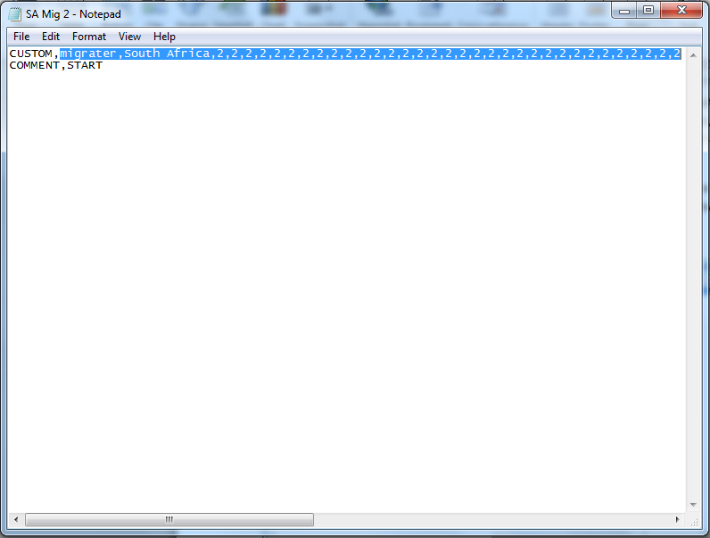
- When copying the code from the .sce to the .DAT file, be sure NOT to include, “CUSTOM,” “COMMENT,” and “START.” See the following example. The .DAT file should only include the highlighted script:
- Once the IFsXXX.DAT file is done, users will have to delete the broken-out model and re-subregionalize. The process will incorporate the newly created .DAT file into the base case.
Provincial Data Processing
The model executes 4 processes when provinces are added (see Adding Sub-Regions for procedural steps):
- Checks for essential series in IFsHistSeriesXXX.mdb
- Normalizes and fills holes in essential series
- Normalizes base-year values in preprocessor variables present in IFsHistSeriesXXX.mdb when provinces are added
- Estimating values for preprocessor series NOT present in IFsHistSeriesXXX.mdb when provinces are added
The following sections will cover these processes in detail.
Checking the Essential Series
As described in section 1, data for sub-regions in IFs are stored in IFsHistSeriesXXX.mdb. In order for sub-regions to be added, data for the essential series is required. The 4 variables are described below.
| Variable | Definition |
|
GDP2011 |
Gross Domestic Product in 2011 Constant Dollars |
| GDP2011PCPPP | Gross Domestic Product per Capita in 2011 Constant Purchasing Power Parity International Dollars |
| Population | Population in Millions |
| LandArea | Land Area |
When sub-regions are added, the model checks that each sub-region has at least one year of data for each of these required variables. If this is not true, then (1) the specific state/province/department cannot be used, (2) it is excluded from the process, and (3) the system will give a message indicating the problem. With these four series, the shell model is established. The user can add incrementally build upon this by adding more data. Also note, sub-regional data must be for years that are available in the country-level data. For example, if only 2011 population data is available for sub-regions, national-level population data must include 2011 as well.
The model will not break-out if GDP2011 does not have year columns back to 1960, whether or not there is sufficient data to fill all those year columns. The GDP2011 table in the IFsHistSeriesXXX.mdb does not have to have to be structurally identical (have the exact same years) as the GDP2011 table in IFsHistSeries.mdb.
Normalization and Hole-Filling in Essential Series
Due to the special importance of these series, the model normalizes and fills in data across all years for each sub-region. Normalization means it modifies sub-regional values with respect to country-level data. To do this, the model checks the base year (2010) for all sub-regions. If base-year data is not available, it uses the closest available year. The aggregation rules for GDP2011, Population, andLandArea are all SUM, so the model simply multiplies the country base-year value by each sub regional contribution:
Since GDP2011PCPPP is defined as a rate, is filled out a little differently. Here, the sub-regional values are multiplied by their respective weights for Population, then summed for a weighted average. Then a multiplier is computed by dividing the country-level GDP2011PCPPP value by this weighted average. The final normalized data are the product of the multiplier and the sub regional values.
Where POP weight is:
These normalization procedures are important for a couple reasons. First and foremost, they allow the model to produce reasonable forecasts. They also allow the user to use any type of unit for the essential series. This may be quite helpful because sub regional data is often harder to find than national figures, especially PPP data.
Normalization of Preprocessor Variables Present in IFsHistSeriesXXX.mdb When Provinces are Added
For preprocessor (non-essential) variables included in IFsHistSeriesXXX.mdb before adding provinces, base year values are normalized. Variables used in the preprocessor are marked in the field UsedInPreProcessor (formerly ‘UseforProvince’) in the DataDict table in the IFsHistSeriesXXX.mdb. Non-preprocessor variables will not be normalized. In general, normalization is important because the preprocessor draws upon base year (2010) data in order to initialize values of the model run. Simply put, provincial values must be consistent with the values for the total country. The process is similar to what we saw for the essential series. The main difference is that the model only normalizes the base year value. Values for other years will not be changed and no hole-filling occurs. First, the model computes a multiplier for provincial data by dividing the country value in the base year by the weighted average, simple average, or sum (designated by aggregation field) of the provinces. If base year data are not available for the country or provinces, the model looks to the Most Recent column for provinces and country data. Note that this could mean the multiplier is computed with data from different years. Multipliers are calculated as:
Where weight is based on the aggregation rule of the variable (generally GDP or POP):
The computed multiplier is stored in the multiplier field for the series row in the datadict table of IFsHistSeriesXXX.mdb in \RUNFILES.
If provincial data differs significantly from country data, likely due to different units, users can check the ApplyMultAll field of the DataDict table in IFsHistSeriesXXX. This signals the model to apply the multiplier to all previous years of provincial data. This should be done before sub-regions are added.
Estimating Values for Preprocessor Series Not Present in IFsHistSeriesXXX.mdb When Provinces Are Added
For variables used in preprocessor not included in IFsHistSeriesXXX.mdb before adding sub regions, the model jumps to IFsHistSeries.mdb and estimates values across all years data is available at the country level. This can happen 2 ways:
- If the aggregation rule (as seen in the DataDict.mdb, not the DataDict table in IFsHistSeriesXXX.mdb) is SUM then we use the disaggregation rule, usually either GDP or POP, to formulate weighted estimates for sub-regions. Thus, the sum of the estimates will always equal the county value in a given year.
- If the aggregation rule is not SUM, the value at the national level is simply applied to all sub-regions for a given year. These should always be rate variables like total fertility rate and life expectancy.
Experienced users of IFs, or other models, may be familiar with other commonly used estimation techniques, like cross-sectional regression. These techniques are applied when rebuilding the base, not during the process of adding sub-regions. In any case, suppose that fertility data were not available for a particular sub-region, but we had GDP per capita figures for the region. The model would fill in the expected values for a country, based on the sub-region’s GDP per capita. Cross-sectional relationships such as TFR-GDP derive from IFs historical data for all countries. A list of all computed functions used within the model can be found under extended features. All variables can be estimated through a combination of such cross-sectional relationships and national level data.
Data Gathering and Prioritization
With the four-essential series imported and the shell model in operation, the user can begin exploring available data sources to fill other preprocessor variables. While estimate-driven forecasts (from the shell model) are a starting point, they offer limited value to policy-makers. Each time a new series is added to IFsHistSeriesXXX.mdb, the quality of sub-regional forecasts improves becoming anchored less on estimates and more on empirics.
Data Sources
Research on potential data sources for sub-national data is the first step in the data gathering process. Preference should be given to official government sources and census bureau data. Human Development reports frequently provide important sub-national data series and can direct researchers to key data sources. Researchers should search for ministry or department data resources as well because they tend to have the module specific data that is needed. For example, the Department of Energy will likely have energy data available sub-regionally. Provinces may also have their own databases which may be worthwhile data sources. It is better to use a single data source for each module's data. For instance, pulling all education data from a single data source is preferred over using multiple data sources. This is not always possible and having some data is better than no data at all.
Each potential data source should be thoroughly researched before any data is pulled into the model. This will decrease the necessity to pull the same series more than once after a better data source is found. All data sources should be catalogued by the series that are available from the source, the format that the data source is in, the temporal coverage available from the data source, the provincial coverage available, how frequently the data is published, and the overall quality of the data source (eg. is this a trustworthy data source, are there potential errors or problems found in the data, is the data in a difficult to pull format?).
Data Pulling Prioritization
Some series are more important than others to the IFs preprocessor algorithms. Understanding the IFs initialization procedure can help inform the prioritization of data gathering efforts. For each module there are several series that contribute especially heavily to the robustness of the model. Overall, priority should be given to series that impact demography, the economy, and human development. This includes but is not limited to; Age-Sex cohorts, Infant Mortality, Life Expectancy (total, male, and female), Value Added, Land Use, Crude Birth Rates, Crude Death Rates, Urban Population, Imports and Exports, Government Consumption, Government Revenues, Mortality by Cause, Education Years, Education Enrollment Rates, Agricultural Production, and Energy Production/Consumption.
Procedural Elements
The following sections present a guided walkthrough of some of the procedural elements of sub-regionalization in IFs. As such, “the user” will be referred to as “you” for the remainder of the document.
Importing Data and Updating Data in IFs
Updating provincial data is a multi-step process. This walk-through will begin with the assumption that you have found the data and you are ready to introduce it into the model. Do not open your IFs model until you’ve made your data changes. With the model open, your changes will not properly register.
Importing Function for Provincial Data in IFs
IFs version 7.05 introduced a function that allows the user to import provincial data into the model. The process is nearly identical to importing data in the standard 186 country format. You do NOT need to have the model broken out into sub-regions to use this feature. Below are the steps for using this feature.
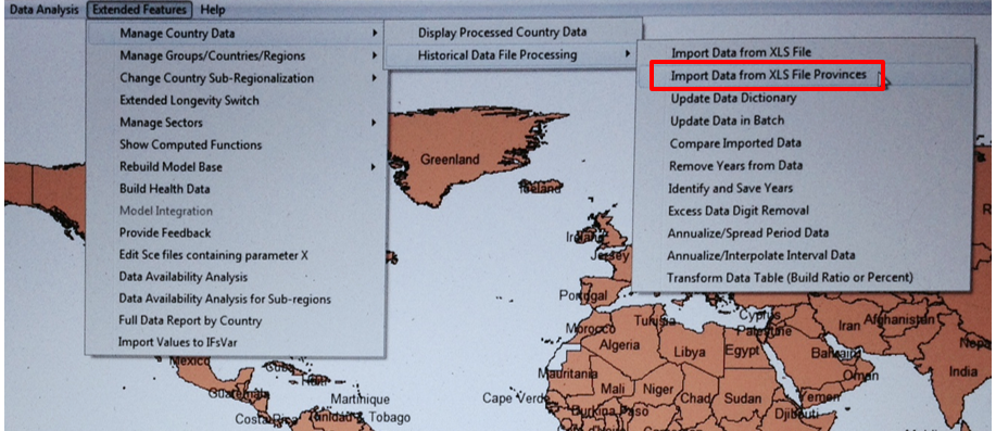
- Open IFs and go to: Extended Features > Manage Country Data > Historical Data Processing > Import data from XLS file provinces
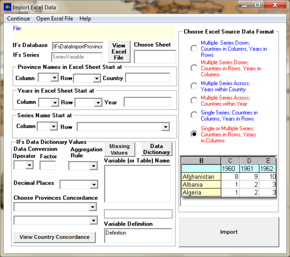
- This brings you to the following window:
- Select Open Excel File and double click the file that has the provincial data you want to import
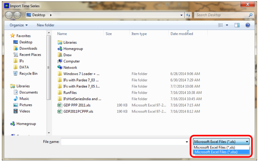
- Note, while the menu path from above says XLS file, this feature can use both XLS and XLSX files. To use XLSX files, you need to use the drop down box located in the bottom right of the Open Excel File window:
- With your file selected, you will be prompted to select the correct Excel Sheet. To see your selected Excel file, click on View Excel. The file will be in read-only mode, so you cannot make changes to the file from here. Make sure to close the Excel file before importing the data, having it open can interfere with the importing process.
- On the right side under Choose Excel Source Data Format the user must select the appropriate data formatting. The bottom option is initially selected by default since most data sets follow this format – State/Province names in rows in rows (vertical) and years in columns. You will notice that the graph below the formatting options changes to visually represent the specific data orientation that you choose
- Next, the user needs to provide the location of state/province names and years in the Excel file. The contents of the selected cell will appear in the blank box to the right of the dropdown menus. Choose the column and row of the state/province name that appears first in your data (e.g. Andaman and Nicobar Islands) and the column/row of the earliest listed year (e.g. 1960)
- Use the dropdown menus to select the appropriate country (e.g. India) and concordance table (concordance tables are covered in next section)
- Under Variable (or table) Name, select the correct variable name for the data (e.g. GDP2011PCPPP). For a new variable, which will be a series that is not a preprocessor series and does not exist in the list of tables, select new. If the variable is new and unit conversion is required (e.g. thousands to millions), user will need to specify an operator and conversion factor. These will automatically be filled in if an existing variable is selected.
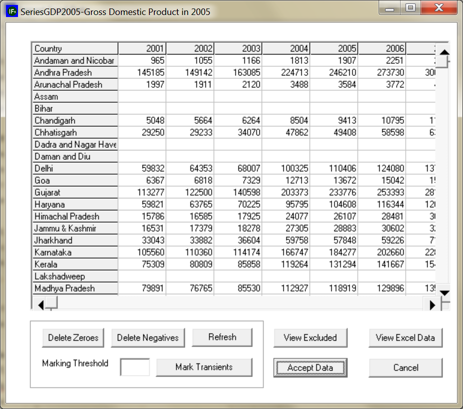
- After completing previous steps and closing the Excel file if it is open, click Import. This will take you to the following window:
- Click View Excluded to see any states/provinces in the source Excel file that were not imported. For example, if one of the listed states/provinces is India, this will be included in the list. It is a common error that state/province names are spelled incorrectly on the source file; this button will alert the user that they need to correct the Excel file and reimport the data.
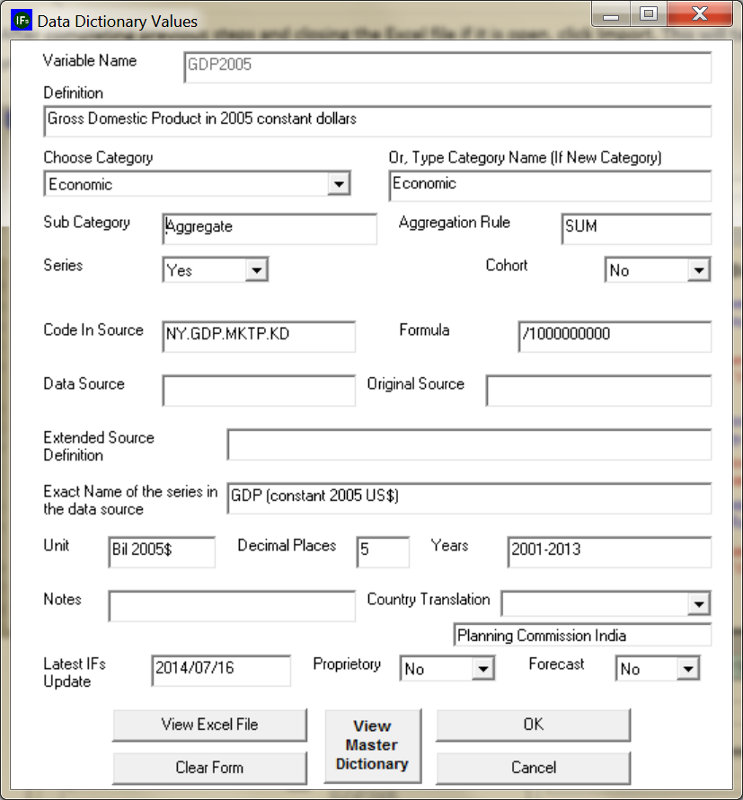
- Clicking Accept will bring you to the data dictionary (datadict) window:
- Again, if an existing variable (not ‘new’) was selected, a lot of this will be filled in. Users will be prompted to fill in required fields after pressing OK if they are blank.
- Imported data can be found here:
- C: > User > Public > IFs > Data > IFsDataImportXXX.mdb
Concordance Tables
Concordance tables are lists that translate the country (or state/province) names found in data source materials to IFs names. For example, if data was being imported from an Excel document from the Indian Planning Commission, the model will import data under the sub-region A & N islands and categorize it as Andaman and Nicobar Islands, the sub-region name in IFs. This saves the user from having to manually translating sub-region names on the source document every time they import new data.
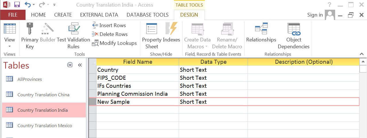
Sub-regional translation tables are located inIFs\Data\Provinces.mdb. To add a list for a new source:
- Open the translation table for the appropriate country
- Click View, located in upper left corner of window, to modify the table design
- In the first blank cell under Field Name, type the name of your new source and select Short Text as the data type:
- Click View again to return to translation lists. Notice the new source now has a column.
- Add the exact sub-region names used in the new source to cells that correlate to the IFs countries. If the new source does not have data for a particular sub-region, leave the cell blank.
- When all sub-regions are entered, save and close Access. Restart IFs and your new concordance list should now be an option in the province data import window.
Manual Import
Users can also manually add provincial data, instead of using the feature within the model. Users can manually import data with any version of IFs, 7.05 is not needed. The data structure of International Futures uses Microsoft Access. For the South African provincial data file, go to:
C: > User >Public > IFs > Data > IFsHistSeries South Africa.mdb
This file is the home to all of the historical provincial data that has been gathered for the provinces (in this case, of South Africa). For the purposes of this tutorial, we will use the example of population.
From the South African 2011 Census, we can now add data for the population total in 2011.
Depending on the data source that you may have, you could want to either change existing data or add a new year of data. Complete the data import process in Microsoft Access before opening IFs.
Adding or Deleting SubRegions
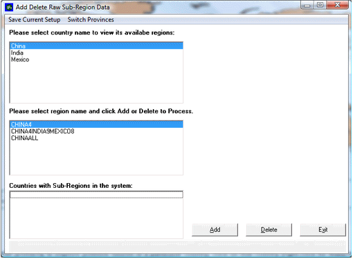
Go to Extended Features > Change Country Sub-Regionalization > Add or Delete SubRegions. This will open the menu below:
With this menu open, select the country name that is desired to be sub-regionalized within the model in the upper-right box within the window. Below this box under Please select region name and click Add or Delete to Process select XXXALL and click on Add. You will be prompted with the following:
Choose Yes this process begins rebuilding the model with the sub-regional breakout. Depending on the processing power of your computer, the first portion of this Add Sub-regions process will take between 3 and 8 hours.
When this is complete, you will be prompted with a window stating Process Complete, select Okay.
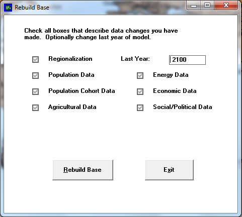
Then the Rebuild Base form should open. Rebuilding the Base Case will place all initial conditions and parameters into the Base Case, but all computed values will be set at 0 until the model is re-run. All boxes on the Rebuild Base form should be checked and the last year should be 2100, then select Rebuild Base.
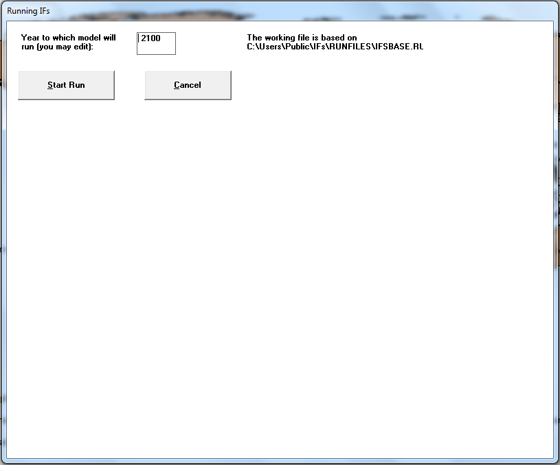
After the base is rebuilt, you should be prompted to run the model with the window below. Run the model to 2100 and select Start Run.
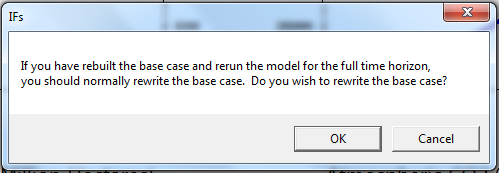
Once the model finishes running to 2100, you will get the message below.
Select OK to this message and then click Run Successful – Click to Continue.
Switching Models
It is also possible to switch between different model runs (i.e. between the national level and a sub-regional model). For instance, you have just completed a sub-regionalization that divides China into single provinces. Now, you would like to use data for the whole country as a Base Case again. To remove all sub-regions, open the window for Add or Delete Subregions. Click on Switch Provinces and choose No State/Province from the right side box of Available Runs. Click Switch to restore the model to pre-sub-regionalization status.
At this point you will be asked if you want to save your current configuration. It is important to select Yes in order switch back to the preferred sub-regionalization the next time you want to revert back to the sub-regional version. This process only takes 5 - 10 minutes, so it is possible to switch back and forth on a regular basis.
Switching Models to Process New Data
To process newly imported data for the preferred sub-regionalization, the existing sub-region setup (used for switching) needs to be removed first and the model needs to be broken out again. To do this users must switch their model from the broken out version to the No State/Province version as described above. The option to delete a sub-region setup is in the same window as to add sub-regions. After the model has been switched to No State/Province select the country from the box on the right, Available Runs: and click Remove to delete the sub-region setup. Deleting a sub-region setup will remove all files created in the process of adding the sub-region setup, and the corresponding model run will no longer be available from the Switch Provinces option.
Appendix
In this example, we will look at how normalized estimates are calculated for Female and Male Life Expectancy (LifExpectMale and LifExpectFemale). Below are abridged datadict entries for the two variables. Since there are values for the Multiplier field, we know this was taken from RUNFILES after sub regions were added. Also, the aggregation rule for the male series was changed from null to GDP for the sake of demonstration. The next steps will detail the steps for calculation the multipliers and the estimated base-year values.
| Variable | Units | Multiplier | ApplyMultAll | Aggregation | UsedinPreprocessor | UseProvData |
| LifeExpectFemale | Years | 0.98 | No | Yes | No | |
| LifeExpectMale | Years | 0.97 | No | GDP | Yes | No |
We will start with the female series. Below is a sample table for what was included in IFsHistSeriesIndia.mdb, along with the 4 essential series (earlier years are left out to save space).
| SeriesLifExpectFemale | ||||||
| Country | FIPS_CODE | 2006 | 2010 | 2011 | Earliest | MostRecent |
| Andaman and Nicobar Islands | AN | |||||
| Andhra Pradesh | AP | 65.5 | 70.9 | 59.8 | 70.9 | |
| Arunachal Pradesh | AR | |||||
| Assam | AS | 59.3 | 64.8 | 51.9 | 64.8 | |
| Bihar | BR | 60.4 | 68.7 | 51.5 | 68.7 | |
| Chandigarh | CH | |||||
| Chhatisgarh | CT | |||||
| Dadra and Nagar Haveli | DN | |||||
| Daman and Diu | DD | |||||
| Delhi | DL | |||||
| Goa | GA | |||||
| Gujarat | GJ | 65.2 | 72.5 | 59.3 | 72.5 | |
| Haryana | HR | 67.3 | 59 | |||
| Himachal Pradesh | HP | 66.3 | 71.3 | 71.3 | ||
| Jammu & Kashmir | JK | |||||
| Jharkhand | JH | |||||
| Karnataka | KA | 67.1 | 72.3 | 62 | 72.3 | |
| Kerala | KL | 76.3 | 77.6 | 71.5 | 77.6 | |
| Lakshadweep | LD | |||||
| Madhya Pradesh | MP | 56.9 | 51.9 | |||
| Maharashtra | MH | 57.9 | 65.3 | 62.1 | 65.3 | |
| Manipur | MN | |||||
| Meghalaya | ML | 68.4 | 72.5 | 72.5 | ||
| Mizoram | MZ | |||||
| Nagaland | NL | |||||
| Orissa | OR | 59.6 | 67.3 | 53 | 67.3 | |
| Pondicherry | PY | 70.4 | 72.8 | 72.8 | ||
| Punjab | PB | 69.6 | 63.6 | |||
| Rajasthan | RJ | 62.3 | 70.7 | 53.8 | 70.7 | |
| Sikkim | SK | |||||
| Tamil Nadu | TN | 67.4 | 71.8 | 57.4 | 71.8 | |
| Tripura | TR | |||||
| Uttar Pradesh | UP | 59.5 | 66.9 | 48.5 | 66.9 | |
| Uttaranchal | UL | |||||
| West Bengal | WB | 65 | 58 | |||
Below is the same table but from RUNFILES after the process of adding sub regions is complete (C:\Users\Public\IFs\RUNFILES). Note two things: 2010 estimates have been added and MostRecent values have been added where appropriate, as highlighted in orange.
| SeriesLifExpectFemale | ||||||
| Country | FIPS_CODE | 2006 | 2010 | 2011 | Earliest | MostRecent |
| Andaman and Nicobar Islands | AN | |||||
| Andhra Pradesh | AP | 65.5 | 69.65 | 70.9 | 59.8 | 70.9 |
| Arunachal Pradesh | AR | |||||
| Assam | AS | 59.3 | 63.65 | 64.8 | 51.9 | 64.8 |
| Bihar | BR | 60.4 | 67.49 | 68.7 | 51.5 | 68.7 |
| Chandigarh | CH | |||||
| Chhatisgarh | CT | |||||
| Dadra and Nagar Haveli | DN | |||||
| Daman and Diu | DD | |||||
| Delhi | DL | |||||
| Goa | GA | |||||
| Gujarat | GJ | 65.2 | 71.22 | 72.5 | 59.3 | 72.5 |
| Haryana | HR | 67.3 | 66.11 | 59 | 67.3 | |
| Himachal Pradesh | HP | 66.3 | 70.04 | 71.3 | 71.3 | |
| Jammu & Kashmir | JK | |||||
| Jharkhand | JH | |||||
| Karnataka | KA | 67.1 | 71.02 | 72.3 | 62 | 72.3 |
| Kerala | KL | 76.3 | 76.23 | 77.6 | 71.5 | 77.6 |
| Lakshadweep | LD | |||||
| Madhya Pradesh | MP | 56.9 | 55.89 | 51.9 | 56.9 | |
| Maharashtra | MH | 57.9 | 64.15 | 65.3 | 62.1 | 65.3 |
| Manipur | MN | |||||
| Meghalaya | ML | 68.4 | 71.22 | 72.5 | 72.5 | |
| Mizoram | MZ | |||||
| Nagaland | NL | |||||
| Orissa | OR | 59.6 | 66.11 | 67.3 | 53 | 67.3 |
| Pondicherry | PY | 70.4 | 71.51 | 72.8 | 72.8 | |
| Punjab | PB | 69.6 | 68.37 | 63.6 | 69.6 | |
| Rajasthan | RJ | 62.3 | 69.45 | 70.7 | 53.8 | 70.7 |
| Sikkim | SK | |||||
| Tamil Nadu | TN | 67.4 | 70.53 | 71.8 | 57.4 | 71.8 |
| Tripura | TR | |||||
| Uttar Pradesh | UP | 59.5 | 65.72 | 66.9 | 48.5 | 66.9 |
| Uttaranchal | UL | |||||
| West Bengal | WB | 65 | 63.85 | 58 | 65 | |
Since no 2010 values were available when the process to add sub regions was initiated, the model looked to the MostRecent column. Next, the model needs to fill in null values, which it does by simply using the national-level base-year value from IFsHistSeries.mdb. In this case, the value for India is 66.675 years, as highlight in orange. Once each state has a usable value, the model reads the aggregation rule from the datadict table in IFsHistSeriesIndia.mdb, as seen above. Since the rule is null, it defaults to a simple average (arithmetic).
|
SeriesLifExpectFemale |
|
|
|
Country |
MostRecent |
|
|
Andaman and Nicobar Islands |
66.675 |
|
|
Andhra Pradesh |
70.9 |
|
|
Arunachal Pradesh |
66.675 |
|
|
Assam |
64.8 |
|
|
Bihar |
68.7 |
|
|
Chandigarh |
66.675 |
|
|
Chhatisgarh |
66.675 |
|
|
Dadra and Nagar Haveli |
66.675 |
|
|
Daman and Diu |
66.675 |
|
|
Delhi |
66.675 |
|
|
Goa |
66.675 |
|
|
Gujarat |
72.5 |
|
|
Haryana |
67.3 |
|
|
Himachal Pradesh |
71.3 |
|
|
Jammu & Kashmir |
66.675 |
|
|
Jharkhand |
66.675 |
|
|
Karnataka |
72.3 |
|
|
Kerala |
77.6 |
|
|
Lakshadweep |
66.675 |
|
|
Madhya Pradesh |
56.9 |
|
|
Maharashtra |
65.3 |
|
|
Manipur |
66.675 |
|
|
Meghalaya |
72.5 |
|
|
Mizoram |
66.675 |
|
|
Nagaland |
66.675 |
|
|
Orissa |
67.3 |
|
|
Pondicherry |
72.8 |
|
|
Punjab |
69.6 |
|
|
Rajasthan |
70.7 |
|
|
Sikkim |
66.675 |
|
|
Tamil Nadu |
71.8 |
|
|
Tripura |
66.675 |
|
|
Uttar Pradesh |
66.9 |
|
|
Uttaranchal |
66.675 |
|
|
West Bengal |
65 |
|
|
|
67.934 |
= mean value |
Lastly, the model needs to calculate the multiplier to be used for normalization. In other words, what value will change the mean to the national value? This is obtained by simply dividing the national value by the mean:
Note this is the multiplier seen in the datadict above. This is multiplied against each MostRecent data point to obtain the normalized values seen in figure 3.
Now, how does this change when the aggregation rule is GDP, as is the case with the male series? The process is the same as the female series through filling null values in the MostRecent column. The national value for males is 63.62 years:
|
SeriesLifExpectMale |
|
|
Country |
MostRecent |
|
Andaman and Nicobar Islands |
63.62 |
|
Andhra Pradesh |
66.90 |
|
Arunachal Pradesh |
63.62 |
|
Assam |
63.60 |
|
Bihar |
68.60 |
|
Chandigarh |
63.62 |
|
Chhatisgarh |
63.62 |
|
Dadra and Nagar Haveli |
63.62 |
|
Daman and Diu |
63.62 |
|
Delhi |
63.62 |
|
Goa |
63.62 |
|
Gujarat |
69.20 |
|
Haryana |
66.50 |
|
Himachal Pradesh |
68.90 |
|
Jammu & Kashmir |
63.62 |
|
Jharkhand |
63.62 |
|
Karnataka |
68.00 |
|
Kerala |
73.20 |
|
Lakshadweep |
63.62 |
|
Madhya Pradesh |
57.00 |
|
Maharashtra |
64.50 |
|
Manipur |
63.62 |
|
Meghalaya |
68.90 |
|
Mizoram |
63.62 |
|
Nagaland |
63.62 |
|
Orissa |
64.30 |
|
Pondicherry |
69.70 |
|
Punjab |
67.40 |
|
Rajasthan |
67.60 |
|
Sikkim |
63.62 |
|
Tamil Nadu |
64.20 |
|
Telangana |
68.60 |
|
Tripura |
63.62 |
|
Uttar Pradesh |
59.40 |
|
Uttaranchal |
66.00 |
|
West Bengal |
69.20 |
Instead of taking the average as was done for females, the model uses a weighted average based on GDP data. In other words, each life expectancy value is multiplied by the state’s proportional GDP contribution to the total GDP for all states, then the resulting values are summed.
|
SeriesLifExpectMale |
|
|
|
|
Country |
MostRecent |
Weights (State GDP/Total GDP for States) |
(MostRecent)*(Weights) |
|
Andaman and Nicobar Islands |
63.62 |
0.001 |
0.04 |
|
Andhra Pradesh |
66.90 |
0.081 |
5.42 |
|
Arunachal Pradesh |
63.62 |
0.001 |
0.08 |
|
Assam |
63.60 |
0.016 |
0.99 |
|
Bihar |
68.60 |
0.028 |
1.94 |
|
Chandigarh |
63.62 |
0.003 |
0.18 |
|
Chhatisgarh |
63.62 |
0.017 |
1.05 |
|
Dadra and Nagar Haveli |
63.62 |
0.000 |
0.02 |
|
Daman and Diu |
63.62 |
0.000 |
0.01 |
|
Delhi |
63.62 |
0.035 |
2.23 |
|
Goa |
63.62 |
0.005 |
0.30 |
|
Gujarat |
69.20 |
0.072 |
5.00 |
|
Haryana |
66.50 |
0.036 |
2.40 |
|
Himachal Pradesh |
68.90 |
0.008 |
0.55 |
|
Jammu & Kashmir |
63.62 |
0.008 |
0.51 |
|
Jharkhand |
63.62 |
0.018 |
1.12 |
|
Karnataka |
68.00 |
0.057 |
3.87 |
|
Kerala |
73.20 |
0.037 |
2.68 |
|
Lakshadweep |
63.62 |
0.000 |
0.01 |
|
Madhya Pradesh |
57.00 |
0.037 |
2.08 |
|
Maharashtra |
64.50 |
0.144 |
9.26 |
|
Manipur |
63.62 |
0.001 |
0.08 |
|
Meghalaya |
68.90 |
0.002 |
0.14 |
|
Mizoram |
63.62 |
0.001 |
0.06 |
|
Nagaland |
63.62 |
0.002 |
0.10 |
|
Orissa |
64.30 |
0.027 |
1.76 |
|
Pondicherry |
69.70 |
0.002 |
0.13 |
|
Punjab |
67.40 |
0.031 |
2.11 |
|
Rajasthan |
67.60 |
0.047 |
3.17 |
|
Sikkim |
63.62 |
0.001 |
0.07 |
|
Tamil Nadu |
64.20 |
0.081 |
5.21 |
|
Telangana |
68.60 |
0.041 |
2.81 |
|
Tripura |
63.62 |
0.002 |
0.16 |
|
Uttar Pradesh |
59.40 |
0.083 |
4.94 |
|
Uttaranchal |
66.00 |
0.012 |
0.77 |
|
West Bengal |
69.20 |
0.064 |
4.42 |
|
|
|
Total = |
65.69 |
The last step is the same as before. What value will change this weighted average to the national average?
Once again, this is the multiplier seen above. This is used to transform each MostRecent data point into a normalized 2010 value.
